
Contents
Install and startupWindows computersMac computers (OS X)Linux computersStarting Chrombox D from the Matlab desktop (on all systems)Changing settingsUpdatingTutorial 1. Least squares spectral resolution (LSSR)1.1. Starting the program1.2. Loading the data1.3. Basic viewing options1.4. Generating a library of compounds1.5. Generating a mass spectral library1.6. Quantification by LSSR1.7. Chromatographic resolution1.8. Other samples.Tutorial 2. LSSR on high resolution direct infusion data2.1. Importing the data2.2. Setting appropriate conditions for filtering and binning.2.3. Creating the library2.4. Quantifying the data2.5. Using the library as a filter.Tutorial 3. The Lipid Gerator 3.1. Basics3.2. Codes3.3. Main functions of the generator3.4. Generation of compounds and filtering3.5. Editing lists for each class3.6. User defined fatty acid lists3.7. Saving and loading settings and compound lists3.8. Sphingoid basesTutorial 4. The profile analyzer4.1. Initialization4.2. Description of functions4.3. Using the functions4.4. Generating a centroided spectrum and resolving it by LSSR4.5. Further description of the functions in the Analyze profile windowTutorial 5. Least squares resolution of profiles (LSSR-P)5.1. Principle5.2. Low resolution data5.3. High resolution dataTutorial 6. Accurate mass determination6.1. Low resolution data6.2 High resolution dataAppendix 1. List of lipid classes with examples of naming
The following text styling is applied in this document. Commands, paths or filenames are denoted by: command, or path\filename.ext. Buttons in the graphical user interface are shown as [Button]. Keys on the keyboard are denoted by [Key]. A parameter to be set is denoted by parameter, and a value of a parameter or an option in a menu is denoted by option.
Install and startup
Quick start
On Windows computers with Matlab you can usually just move the folder
DDto your preferred destination and start the program by double click on theChrombox D.exefile.Follow the instructions below if you install on a Mac or Linux computer, or if you install the program on a network drive.
Windows computers
Download the installation and unzip the archive
dd.zipMove folder
DDto the preferred destination, e.g.C:\CHROMBOX\. This will be the D-root folderIf Installed on a local disk or on a memory stick, Chrombox D can usually be started by using the
"Chrombox D.exe"file in the D-root folder.
If installed on a network disk, you may have to use one of the methods described below:
Find the file
dstart.min the folder…\dd\variousand move it to somewhere in your Mathlab path. This is the only file that needs to be in the Matlab path. Possible destinations may be found by starting Matlab and typingpath.Open the
dstart.mand edit the last line after theruncommand, so that it points to the filedd_startscript(see example below).You should now be able to start Chrombox D by typing
dstartin the Matlab command window.
An example of dstart.m is shown below:
x% Startupscript for Chrombox D% Starts startscript by the run command.% Startscript must be located in the D root, % dstart must be in the matlab searchpath% run c:\DD\dd_startscript
run C:\CHROMBOX\DD\dd_startscriptYou can also create a desktop shortcut by copying the shortcut to Matlab and adding the following to the destination: /automation /r dstart. An example of how it can look is shown below:
C:\MATLAB6p5\bin\win32\matlab.exe /automation /r dstart
Mac computers (OS X)
Download the installation and unzip the archive
dd.zip.Move the folder
DDto the preferred destination, for example/Users/yourname/Documents/CHROMBOX/DD, This will be the D-root folder.The shell script
macstart_d.commandstored in the D-root folder can be used to start the program if the file is executable and Matlab can be started with the terminal command./matlab. Note that the extension.commandmay be hidden in Finder.To check if Matlab can executed by
./matlabopen the terminal and type./matlab. If Matlab does not start you can do the following:Put a symbolic link to Matlab in your path by opening the terminal and typing
sudo ln -s /Applications/MATLAB_RXXXXx.app/bin/matlab /usr/local/binwhereRXXXXxshould be replaced by the Matlab version number, for example "R2017a". Alternatively, openApplicationsin Finder. Locate Matlab, right-click and selectShow Package Contents. Open the folderbinand locate the application filematlab. In terminal typesudo ln -swithout pressing enter. Thereafter drag thematlabapplication file to the terminal. Ensure there is a space between "-s" and"/Applications"and press enter.
To make
macstart_d.commandexecutable, do the following:Open the terminal. Use
cdto change directory to the D root where themacstart_d.commandis located or open the terminal at the D root folder if that is an option. Typechmod +x macstart_d.command. Alternatively, typechmod +xwithout pressing enter and drag themacstart_d.commandfile from Finder to the terminal. Ensure there is a space between"+x"and"macstart_d.command"and press enter.Thereafter double-click on
macstart_d.commandin Finder to start the program. Depending on your security settings you may get the following message: "macstart_c.command can’t be opened because it is from an unidentified developer". To solve this, open System Preferences – Security and Privacy – General and press[Open anyway]next to the message regarding the file. An alternative way of allowing the file to be executed is to open the file in TextEdit and saving it again. Then it will no longer have status as downloaded from the Internet.
As an alternative to the above procedure, Chrombox D can be started by the following method:
Find the file
dstart.min the folder…/dd/variousand move it to somewhere in your Matlab path. Possible destinations may be found by starting Matlab and typingpath.Open the
dstart.mand edit the last line after theruncommand so that it points to the filedd_startscript(see example below).You should now be able to start Chrombox D by typing
dstartin the Matlab command window.
An example of dstart.m is shown below:
xxxxxxxxxx% Startupscript for Chrombox D% Starts startscript by the run command.% Startscript must be located in the D root,% dstart must be in the matlab searchpath% run C:\DD\dd_startscript
run /Users/yourname/Documents/CHROMBOX/DD/dd_startscript.m
Linux computers
Download the installation and unzip the archive
dd.zip.Move folder
DDto the preferred destination, for example/home/yourname/CHROMBOX/DD, This will be the D-root folder.The shell scripts
linstart_d.shstored in the D-root folder can be used to start the program, if the file is executable and Matlab can be started with the terminal commandmatlab.On Ubuntu you can use the following procedure to make
linstart_dexecutable:Right-click on the file and select
Properties. SelectPermissionsandAllow executing file as program.
It should now be possible to start Chrombox D by double-click on
linstart_d.shand selecting the optionrun in terminal. If you don’t get therun in terminaloption while double-clicking the file you will have to edit the preferences in the file manager. ChooseEditin the menu for Files, thereafterPreferencesand select theBehaviourtab. SelectAsk each timeas the option for executable text files.There is also a file
linstart_d_term.shin the D-root folder. The difference betweenlinstart_dandlinstart_d_termis that linstart_d runs the application disconnected from the terminal whilelinstart_d_termruns in the terminal. Chrombox D will continue to run if you close the terminal if it was initiated bylinstart_d, while it will close together with the terminal if it was initiated bylinstart_d_term.
As an alternative to the above procedure you can also start Chrombox D by dstart.m as described for Mac computers above.
Starting Chrombox D from the Matlab desktop (on all systems)
On all operating systems you can use the following procedure to start Chrombox D:
Start Matlab in the regular way, so that the Matlab desktop is opened.
Change the current working directory of Matlab to the D-root folder, either by the line showing the working directory or by browsing in the panel in the left side of the Matlab desktop.
You can now start Chrombox D by one of the following methods:
Select
dd_startscript.min the panel showing the contents of the working directory, right-click and selectrun.type
run dd_startscriptin the Matlab command window.
In a minimized Matlab session (running in terminal without Matlab desktop) you can use the cd command to set the working directory and run dd_startscript to start the program.
Changing settings
The program should normally start without the need to change any settings. But you may want to adjust parameters such as window size. These are specified in the
dd_localsettingsfile in the D-root folder.Open
dd_localsettings(.sdv or .csv) in an editor such as Notepad and edit the paths for raw data, etc, if necessary.An example of “dd_localsettings” is shown below. Parts to check or edit are shown in blue.
xxxxxxxxxxdefaultfolders;1; Specifies whether the default setup for folders is used (1 or 0, use 1 for simple setup)version;D-12-09b; Code version and name of subdirectory for codesdefaultmethod;Default; Method to load on startwindowpos;[0.1 0.1 0.75 0.75]; Position and size of main windowpath_cdf;K:\CHROMBOX\DD\cdf; Path for NetCDF filespath_mzxml; K:\CHROMBOX\DD\mzxml; Path for mzXML files.path_....path_....user;Anonymous; Specify user signature for info filestracker;0; For development purposes
windowposis position of the window in fractions of the screen size. The two first numbers in the vector is the position of the lower left corner. As specified above the lower left corner is 10% from the bottom of the screen and 10% from the left. The height and width is 75% of the screen size. Ensure that the sums of numbers 1 and 3 and numbers 2 and 4 are less than 1.If
defaultfoldersis set to 1 the program will use the standard setup for subfolders and it is not necessary to edit the paths even if they are not correct. If the parameter is set to 1 you will have to specify the location of each path for data and methods. Data can be read from other folders than the ones are specified. Folders can also be changed by using the[Settings]option within the program.versionrefers to the current version of the code. The parameter can also be updated from within the program.If you have created a method that you want to import on startup you specify this as
defaultmethod.
Updating
Download the new version from www.chrombox.org/D
Unzip the archive with the new code.
The folder containing the code, e.g.
D-12-06should be placed in the foldercodein the D root folder..Open the file
dd_localsettings.sdv(may also have .csv extension) that is found in the D root folder and update the version to the folder name of the new code. The part to be edited is shown in blue in the example below.Note that it is not necessary to delete the folders with old code. Keeping these allow you to run previous versions if necessary.
An example of dd_localsettings.sdv is shown below. The part to edit is between the two semicolons in the first line.
xxxxxxxxxxversion;D-12-06b;Current version and name of subdirectory for codesdefaultmethod;Default;Method to load on startwindowpos;[0.1 0.1 0.75 0.75];Position and size of main windowpath_cdf;K:\CHROMBOX\DD\cdfuser;Anonymous;Specify user signature for info filestracker;0;For development purposes
Alternatively, you may select the new code by the following procedure:
Open Chrombox D
Press the
[Settings]button down in the right cornerSelect
[Load/Files]Select the code version and press
[Save local settings]Restart Chrombox D.
Tutorial 1. Least squares spectral resolution (LSSR)
The purpose of this tutorial is to learn basic features of the program and how to quantify samples using least squares spectral resolution (LSSR). The samples are unit-resolution LC-MS data of phosphatidyl cholines (PC) and sphimgomyelins (SM) analyzed by precursor ion scan of m/z 184. Details of the methodology are given in Zeng et al., J. Chromatogr. A 1280 (2013) 23.
1.1. Starting the program
Start by opening the main window, by writing “dstart” in the Matlab command window, by starting the
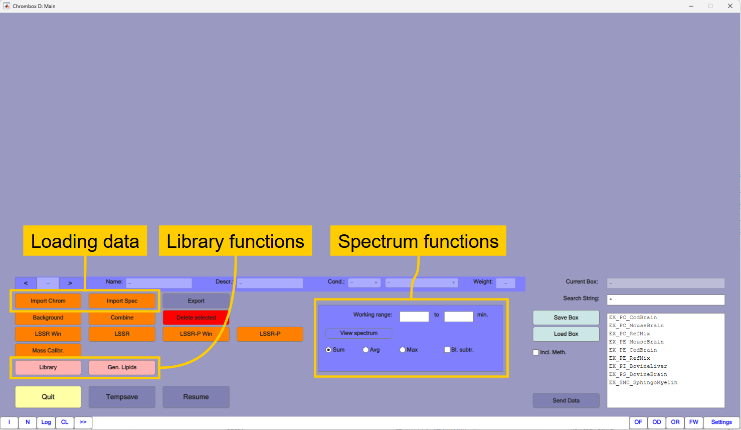
Chrombox D.exefile in the D root folder (i.e.C:\CHROMBOX\DD), or as described in the installation instructions for Linux and Mac. The main window should look like Figure 1.1.
You will need functions for loading data, for creating libraries and for handling spectra.
1.2. Loading the data
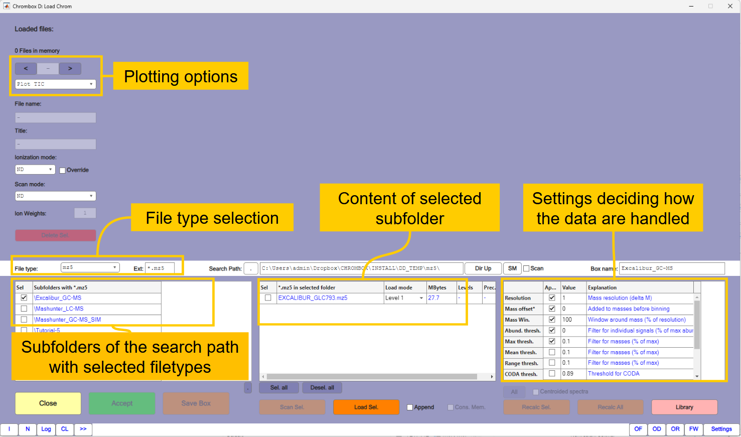
Press the
[Import Chrom]button that takes you to the window for importing chromatographic data shown in Figure 1.2.Ensure that the selected file type is NetCDF
Select the subfolder
\Tutorial-1and select all four files in the subfolder.PCs typically have masses in the middle between two unit resolution masses, which can cause problems when the raw data masses are rounded to integer values. To ensure that all masses are rounded in the same direction you must set the mass offset in the table to the right to 0.2. This adds 0.2 to the original masses before rounding. Leave the other settings in the table at default values. More information about these settings are given in Tutorial 2.
Press thereafter
[Load Sel.]to load the four files.You can inspect the files by selecting files and plot types in the plot options in the upper left corner of the window.
Press
[Accept]when finished. The chromatograms should now appear in the main window.
1.3. Basic viewing options
In the main window you can you can choose between displaying the total ion currents (TIC) and individual ions by using the radio buttons to the right in the line below the chromatograms. Right-click in an ion-chromatogram will give you additional options. You can navigate in the chromatogram by the [+] and [-] buttons and by the slider next to them.
The chromatograms are selected by the
[<]and[>]buttons on the next line.Right-click in a chromatogram gives you the option to view a spectrum at a certain retention time.
You can also view the spectrum of a region of the chromatogram. Select the first chromatogram. Type in
14to47min in the working range in the "Spectrum functions" area (See Fig. 1.1). ChooseSumand press the[View Spectrum]button. This will display the sum of signals of the selected region. The spectra can be exported graphically or numerically by right-click in the figure.
The region to display can also be changed by right-click on the vertical dotted bars in the chromatogram.
1.4. Generating a library of compounds
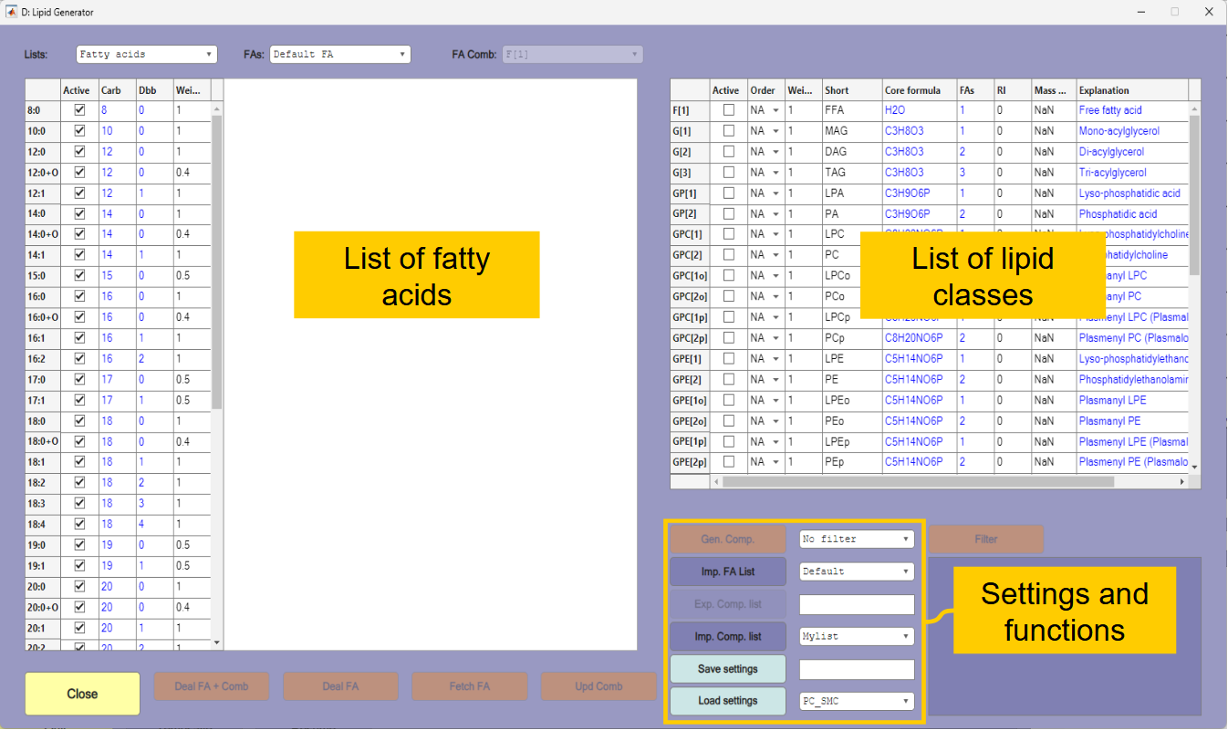
The purpose of this exercise is to identify PC species in the four samples. For that you will need a library of compounds and spectra that can be found in the samples. The compounds are generated by the Lipid Generator function that is opened by the [Gen. Lipids] button in the main window. The lipid generator generates possible lipid compounds based on lists of fatty acids, sphingoid bases and the lipid class core formula.
The window of the lipid generator is shown in Figure 1.3. When using the function it is important to consider which fatty acids, sphingoid bases and lipid classes it is possible to have in the analyzed samples – and which that can be detected under the experimental conditions that was applied. Although many of the fatty acids and sphingoid bases in the list are not expected to be abundant in the samples, there is no need to make changes to the default lists in this case. The applied MS conditions (precursor ion scan of m/z 184) means that only choline containing compounds are detected. These must therefore be selected in the lipid class list to the right in the figure.
Select the following lipid classes in this order:
GPC[2](ordinary PC),SPCF(Choline containing sphingomyelin),GPC[2o](PC plasmalogen with ether bond),GPC[2p](PC plasmalogen with vinyl-ether bond).Set the filter next to the
[Gen. Comp.]button toWeights. This will ensure that isomeric compounds are not generated. If isomers occur, the one regarded as most likely (based on weights of fatty acids and the order of generation) will be preferred.Press
[Gen. Comp.]to generate the compounds. This will create a compound list with approximately 730 unique molecular formulas. Possible isomers of each compound are listed in the rightmost column. You may get additional information about a molecule by selecting it in the list and searching for instance LipidMaps or EMBL by using the popup-menu that appears under the list. Navigation in the table may be more convenient if you right-click in the table and changes the view toList view.Save the compound list by typing
Tutorial-1next to the[Exp. Comp. List]button and thereafter press the button. The compound list is saved in semicolon separated CSV format and can also be edited in a spreadsheet or a text editor.Close the lipid generator window. Further details about the lipid generator are explained in Tutorial 3.
1.5. Generating a mass spectral library
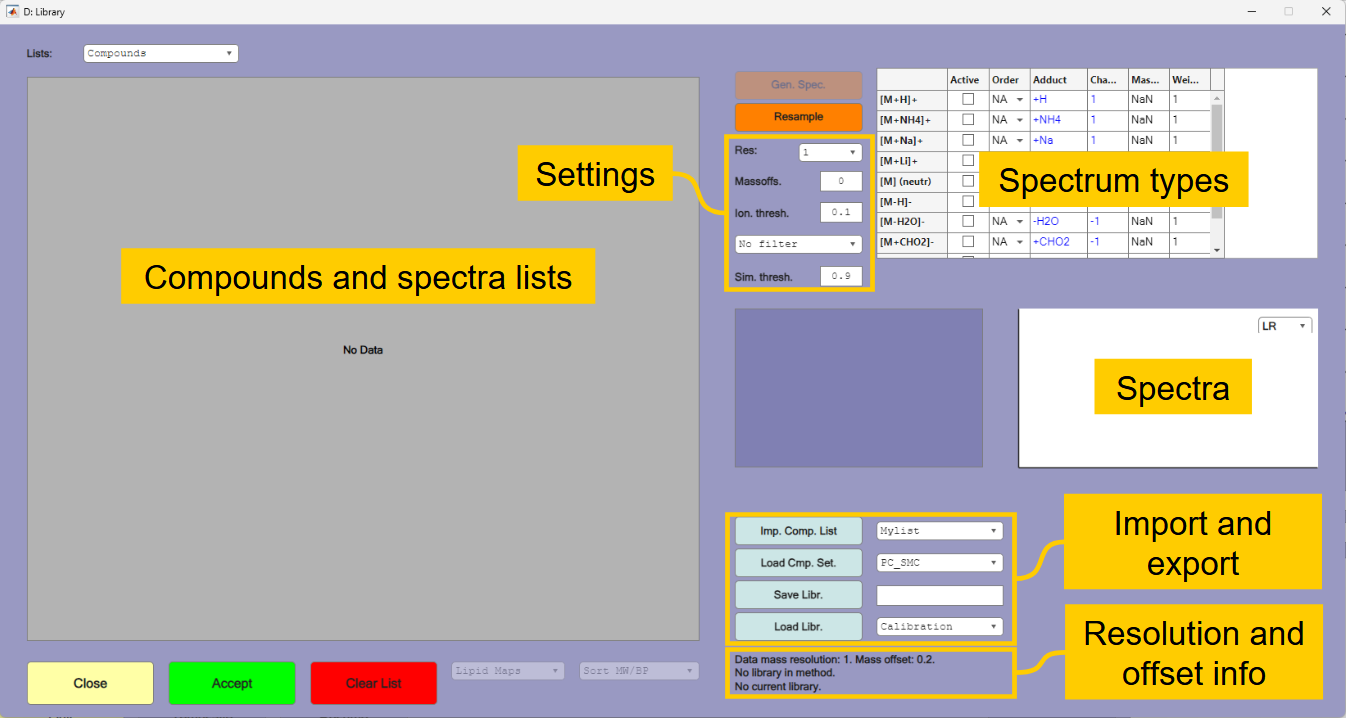
The next step is to create the mass spectral library from the compound list. Press the [Library] button in the main window. The library window is shown in Figure 1.4. The library window will import and display the library that is currently in the method when opened. When the list is empty, as in figure 1.4, it means that no library is stored in the method.
Select your created compound list
Tutorial-1in the popup menu next to the[Imp. Comp. List]button and press the button to read the list.
Before generating the spectra, you must pay attention to the information given by the resolution and offset info. This tells that the data currently in memory has a resolution of 1 and a mass offset of 0.2. The resolution of the data and the generated spectra should usually be identical. In most cases the mass offset should also be identical. The exception is if mass offset is used to compensate for a systematic deviation in the mass accuracy of the instrument.
Change the
mass offsetin the settings to0.2and also changeNo filtertoWeights. The other settings can be kept at default values.
The next step is to select the spectrum types to be generated. The function can generate several spectra, but in this case all relevant ions have positive H+ adducts.
Select the
[M+H]+option in the list of spectrum types.Press thereafter
[Gen. Spec.]to generate spectra with the isotope distribution of the compounds.
The spectra are first generated with resolution of 0.001 and thereafter downsampled to the required resolution and mass offset. In the list of generated spectra there are some that are set as not being "active". These are of compounds with very similar spectra to other compounds in the list; the correlation between the spectra is higher than the similarity threshold of 0.9. These will not be applied by the LSSR algorithm. Which of the similar spectra that will be set as active is decided by the weights that are inherited from the compound list. You may change these selections, but only one of the interfering spectra should be set as active at any time. With a higher mass resolution you would have experienced fewer interferents.
You can view the spectra in high or low resolution by selecting them in the list.
You can save your generated library by typing
Tutorial-1in the field next to the[Save Libr.]button and thereafter pressing the button.Press
[Accept], which will transfer the library to the method and close the library window.
1.6. Quantification by LSSR
The next step is to quantify the compounds using LSSR. Select the first chromatogram (CODBRAIN_PC) and ensure that the selected region marked by the vertical dotted bars spans the region of the chromatogram where there are signals (Approx 15-47 min).
Press the orange
[LSSR win]button that will take you to the least squares spectral resolution window. The spectrum is resolved as long as there is a library in the method and the resolution of the library fits the resolution of the data. The window should look approximately like in Figure 1.5.
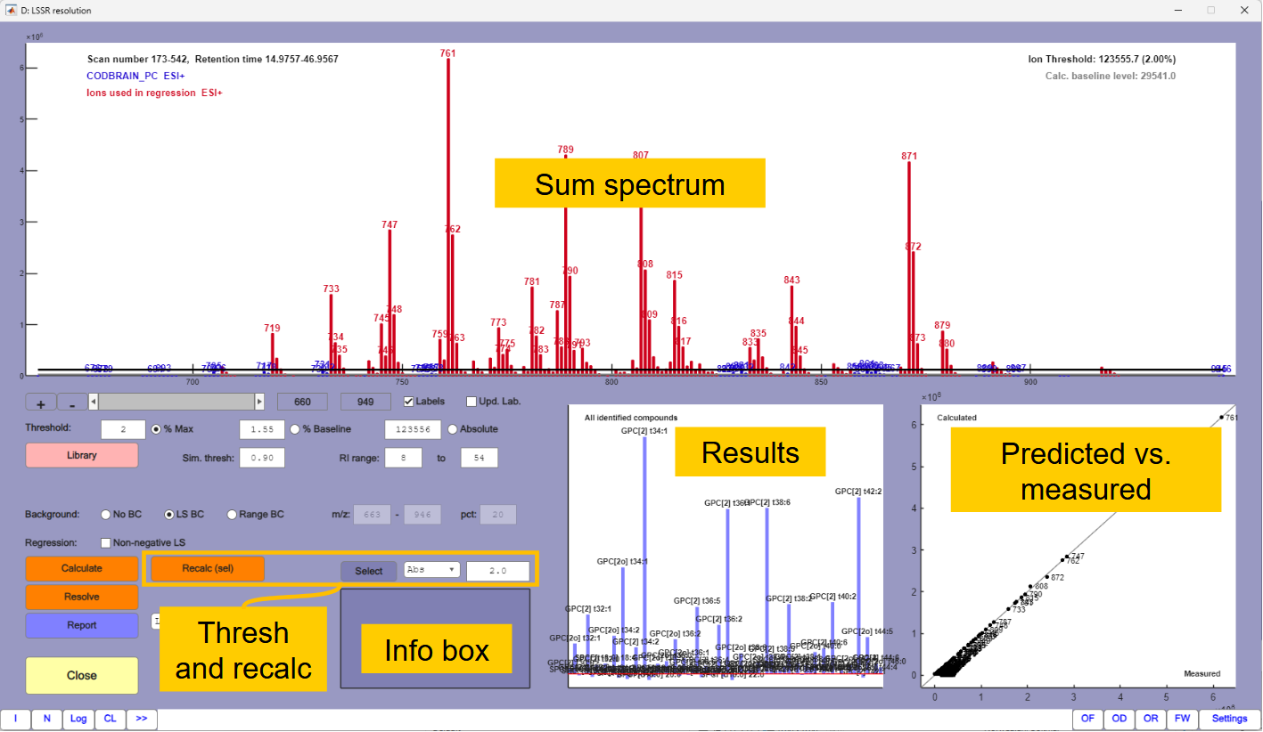
There are three plots in the window. The main plot is the sum spectrum of the selected region. The horizontal black line is a threshold (in this case set to 2% relative to the most abundant mass). Compounds that do not have a base peak above the threshold are excluded from the calculations. Red masses are masses in the compounds that are included in the calculations. Any green masses (none in this case) are masses that are above the threshold, but that do not match any active compounds in the library. Other masses are blue. The horizontal grey line is a baseline estimate. This level is subtracted from all masses in the regression.
The predicted versus measured plot shows how well the calculated solution explains the spectrum. Any severe deviations (none in this case) show that the masses are not properly explained. Right-click on a deviating mass will show which compounds the mass belongs to. The compounds may not be accurately estimated if there are severe deviations between predicted and measured values of the masses.
The third plot shows the total signal from each compound detected. There will usually be a large number of bars with low levels and also some negative values because of noise and baseline subtraction. It will therefore usually be necessary to do a recalculation after selecting a proper threshold level.
Type
2in the edit field next to the[Select]button and thereafter press the button. This will mark compounds that are above 2% relative to the most abundant. Press thereafter[Recalc (sel)]. This will recalculate the abundances using only compounds that were above the selection threshold, and the plot will be simplified. To better view the plot you can right-click on the background and selectCopy figure. The result should look approximately like in Figure 1.6.

The majority of the compounds belong to the GPC[2] class, which are ordinary prosphatidyl cholines. “[2]” indicates that two fatty acids are bound to the molecule and the numbers that follows “t” indicate total number of carbons and total number of double bonds in the two fatty acids. There are also some compounds belonging to the GPC[2o] class indicating that one of the fatty acids is ether-linked (plasmalogens) and a few minor compounds belonging to the SPCF class (sphingomyelins). It should be emphasized that the identities are the one the program regard as the most likely, based on the weights of fatty acids and compound classes, and that there may be several alternative explanations.
If you right-click on the GPC[2o] t34:1 marked by the red arrow in the figure you will be told that the compound has a base peak of 747. Press the
[Library]button, which will open the library, and scroll down to the compounds with base peak of 747 in the spectrum list. You will see that there are three compounds with this base peak and only one is active. Assume that you have reason to believe that this peak is the GPC[2] t33:1. Set this peak as active and GPC[2o] t34:1 as inactive and leave the library window by pressing[Accept]. Press thereafter[Calculate]in the LSSR window, press the[Select]button again with a threshold of 2, and press[Recalc. (sel)]. The identity of the compound should now be GPC[2] t33:1.You may get additional information by searching LipidMaps and other sources. Right-click on the compound in the bar plot and right-click thereafter in the Info field. This will give you options for looking up the molecular formula on the web. The alternatives that do not contain a choline group can be disregarded in this case because of the acquisition parameters.
Results can be reported by pressing the [Report] button. The report format can be selected by pressing [Settings] down in the right corner and thereafter [Reports].
1.7. Chromatographic resolution
Since the data is LC-MS data you can perform a chromatographic resolution based on the theoretical spectra of the compounds that is shown in the bar plot.
Press
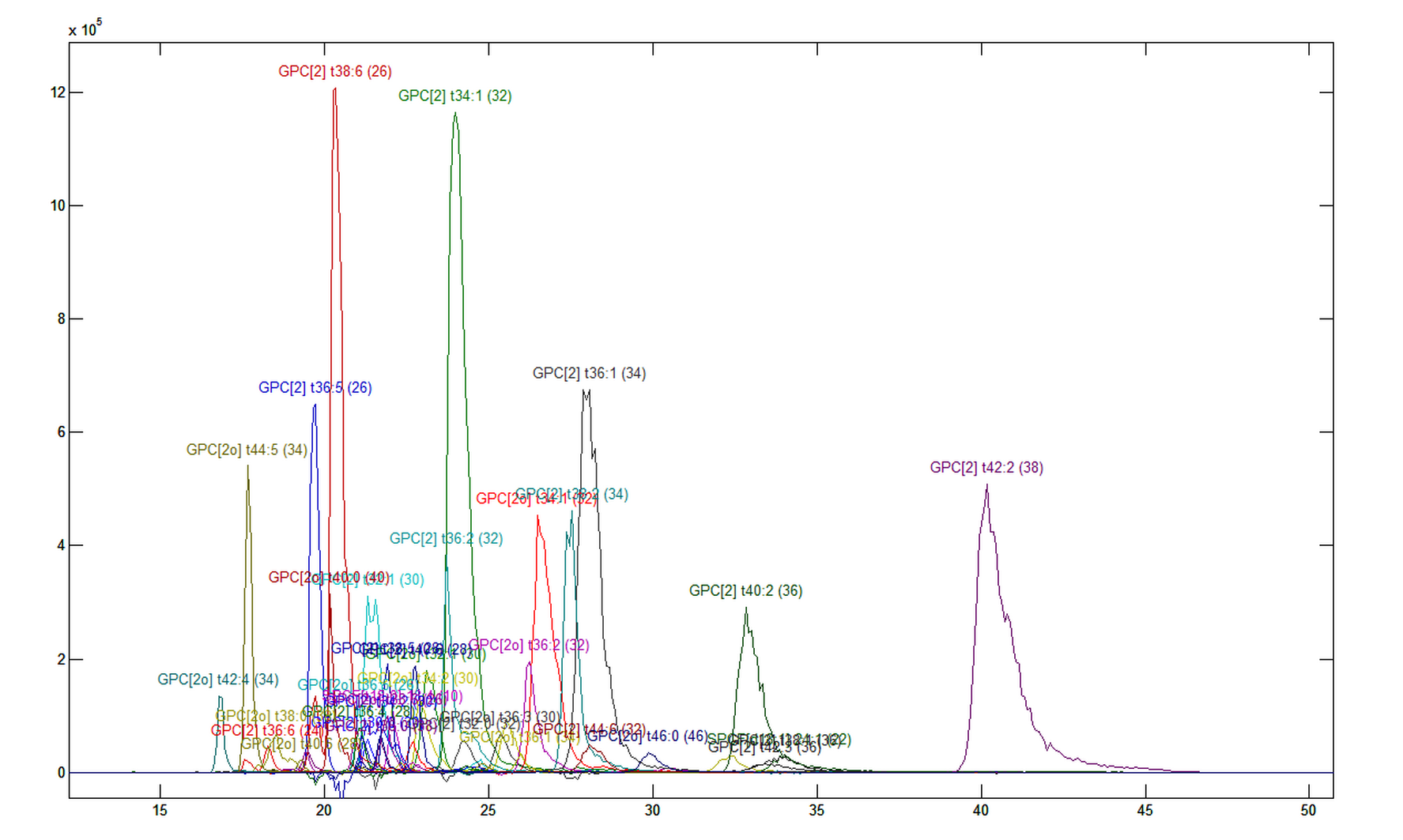
[Resolve]in the LSSR window and[Subtract BL]in the resolution window.
This should give you a resolved chromatogram similar to the one in Figure 1.7. The numbers in brackets behind the identities are equivalent carbon numbers (ECN). Peaks belonging to the same class and with the same ECN should be grouped together. Severe deviations from this pattern may indicate incorrect identification. Clicking on a peak or on a label will highlight the peaks. You may see that some profiles have double-peaks, which indicates that there are several isomers.
1.8. Other samples.
Close the Resolve and the LSSR windows. Change the chromatogram to number 2 “Mousebrain PC” using the
[>]button in the main window. Adjust the vertical bars so they fit the region of the chromatogram with signals and repeat the LSSR procedure. Do the same for chromatogram 3 and 4.
In chromatogram 2 and 3 you can see that several of the major components consist of more than one isomer (e.g. GPC[2] t36:4 at approx 28 min). Some of the peaks late in the chromatogram are sphingomyelins (SPCF).
Chromatogram 4 is a reference mixture of sphingomyelins. All major peaks belong to the SPCF group. Note that there are several isomeric compounds in the SPCF group, so the displayed identities may not be correct. In addition, low resolution mass spectrometry cannot distinguish between compounds such as SPCF[d18:1] 18:0 (C41H83N2O6P) and SPCF[t17:1] 18:1 (C40H79N2O7P). If you have knowledge about which sphingoid bases you can expect in your samples you can avoid many of these conflicts by deactivating or downweighting compounds in the list of sphingoid bases in the Lipid Generator. Four common sphingoid bases are set as active by default. These are d18:1 (Sphingosine), d18:0 (Sphinganine), t18:1 (Dehydrophytosphingosine) and d17:1 (C17 Sphingosine).
Tutorial 2. LSSR on high resolution direct infusion data
The purpose of this tutorial is to learn how to apply LSSR with high resolution direct infusion data, and how you should read in the data with best possible quality.
2.1. Importing the data
Start the program as explained in Tutorial 1, open the window for reading chromatographic data by pressing
[Import Chrom]and selectmzXMLas the file type.In the left table, select the folder
/Tutorial-2and thereafter selectSM_INFUSin the middle table.Thereafter press the
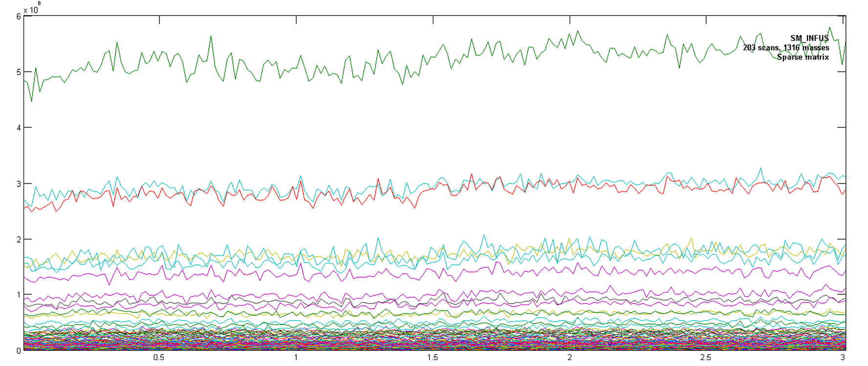
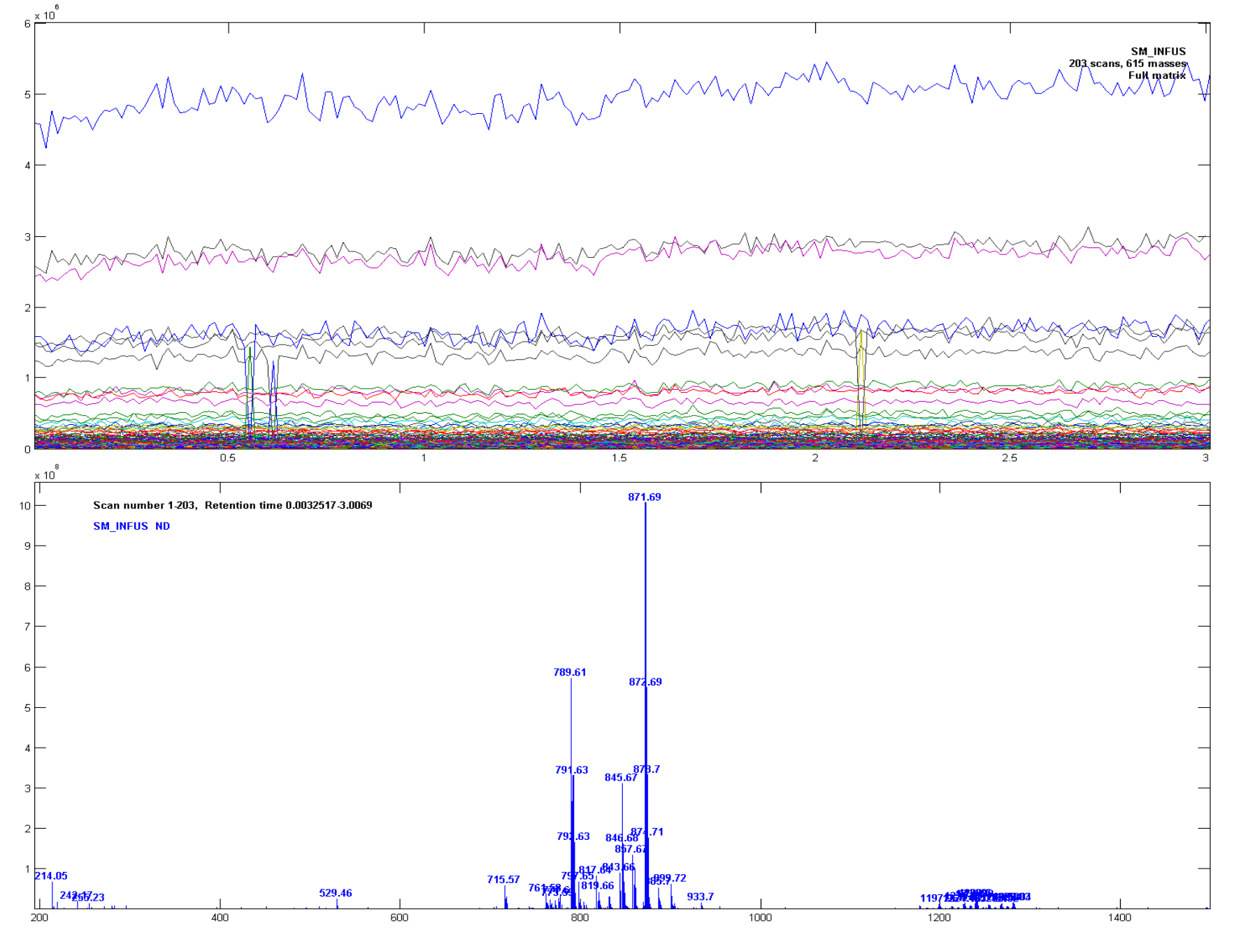
[Load Sel.]button to read the file.Select the
Ions Chromamong the display options in the upper left corner of the window. The ion traces should look like in Figure 2.1.
2.2. Setting appropriate conditions for filtering and binning.
The plot in Fig. 2.1 is of unit resolution data. The unit resolution spectrum can be seen by selecting Avg Spectr as the display option. The data were acquired by high resolution MS, and the next step is to find out how good resolution you can use when the data are analysed, by varying the resolution and mass offset. The resolution in AMU can be any value from 0.001 to 5 that will give an integer value when used as a divisor for 1, i.e. 0.5, 0.2, 0.1, 0.05, ..., 0.001). The offset can be set to any number but it should usually have an absolute value smaller than the resolution.
Ensure that
Ions Chromis selected as display option, type in gradually decreasing values for resolution in the table to the right and press[Recalc Sel.]after each step. From 0.05 you will see that spikes start to appear in the traces because there are masses that are close to the borders of the mass bins, and that some times are rounded up and sometimes rounded down. You may get rid of the spikes by experimenting with different mass offsets. The mass offset is added to the raw m/z values before they are rounded.
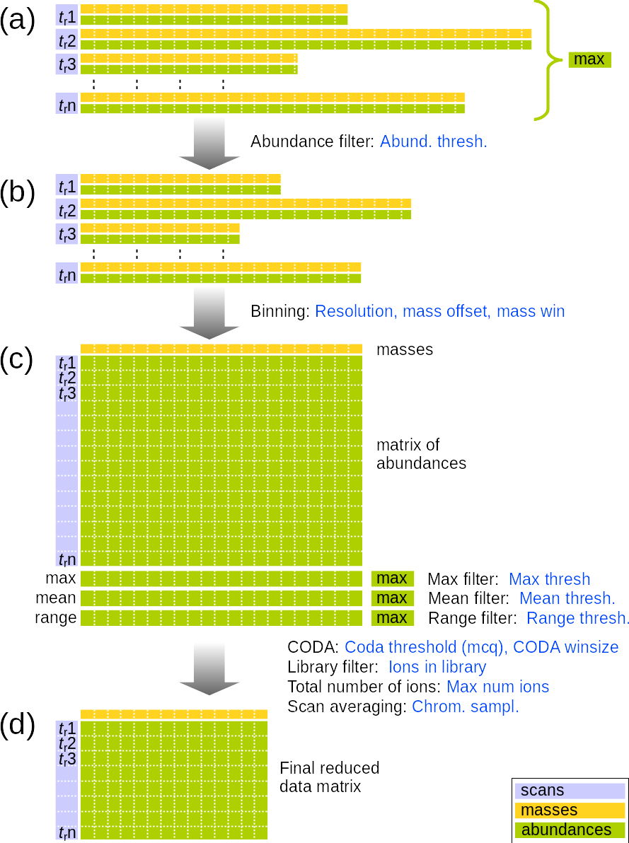
The options for the binning and filtering algorithm is explained in Figure 2.2 and in the text below.
In most MS data files, spectra are stored as pairs of vectors of masses and abundances for each retention time, tr (Fig. 2.2a). These vectors typically vary in number of recorded ions and are without a strictly defined resolution.
The first filter that is applied is the abundance threshold filter that removes low signals that are expected to have insignificant influence on the data. The threshold is given in percent of the largest individual signal in the original spectra. Any signal below this threshold is deleted. The main purpose of this filter is to speed up the binning function and the threshold should normally not be so high that it has significant influence on the final results. The default value for Abund. Thresh is 0.01% of the most intense signal in the data. After application of the filter, the spectra have fewer ions, but the original data structure is kept (Fig. 2.2b).
The next step is the binning function. The purpose of this is to organize the spectra into a matrix of intensities where each entry in the matrix corresponds to the signal from a defined mass and a defined retention time (Fig. 2.2c). This is controlled by the parameters Resolution, Mass offset and Mass win. Resolution is the selected mass resolution in AMU in the final data matrix. Mass offset is a value that is added to the original masses (from Fig. 2.2b) before they are rounded to the required resolution. Mass win is the window size of the binning algorithm. This 100% by default, which means that all signals that pass the Abund. Thresh. filter will contribute to the binned signal matrix. This can be constrained to leave out masses that are between the expected signals. If the window is set to 100% and the resolution is 1, all ions between m-0.5 and m+0.5 are assigned to m, and all ions between m+0.5 and m+1.5 are assigned to m+1. If it is set to 50%, all ions between m-0.25 and m+0.25 are assigned to m and all ions between m+0.75 and m+1.25 are assigned to m+2. This means that signals from ions between m+0.25 and m+0.75 will not be recorded.
Each column in the signal matrix corresponds to an ion trace. After the signal matrix is constructed, vectors containing the maxima, means and the ranges of each column in the matrix are calculated. These values are compared to the maxima of each of these vectors by the max, mean and range filters. The threshold values for these are percents relative to the max value in each of the vectors of corresponding values. Ions that do not pass any of the active filters are deleted. When applying these filters it is important to consider which type of data one are working with. Important ions in chromatographic data can be expected to have a maximum well above baseline and a certain difference between the max and min values, so it makes sense to apply the max and the range filters. The mean filter may be an efficient way to remove spikes because a single spike in the signal will have little influence on the overall mean of the signal. However, this is also the case for small and narrow peaks, so the filter should therefore be used with care with chromatographic data. On direct infusion data, as applied in this tutorial, one should expect intensities to be fairly stable. A range filter therefore makes little sense and the mean filter may work better than the max filter, which is why the mean filter should be active in this case and the two other should be unchecked.
Three more optional filters that work on the ions can be applied. CODA is a method for detecting relevant signals in chromatographic-mass spectrometric data [Windig et al., Analytical Chemistry 68 (1996) 3602-3606] and the parameters that control it are the CODA Thresh. and CODA winsize. You can also constrain the ions to only those that are in the library compounds if there is a library in memory. When applying the library filter it is important that the library has the same resolution as the data, and the mass offset should usually also be the same. You can also set a maximum number of ions to return. If this filter is used, it returns the ions with the largest maxima in the ion traces. By default the filter is active and the maximum number of ions are 5000.
Finally, the data matrix can be resampled in the chromatographic direction by summarizing two or more scans. The final result can be a data matrix (Fig. 2.2d) that is reduced both in the chromatographic and the spectral direction.
You can test how different filters and conditions affect the data. Inspect both the ion chromatograms and the average spectra.
In the following sections it is assumed that the data were sampled with a resolution of 0.01, a small negative mass offset of -0.001, Mass win. of 100%, Abund. thresh. of 0.01%, Mean threshold of 0.1%, and all other filters turned off. The ion trace and the average spectrum with these conditions are shown in Figure 2.3. There are still a few negative spikes, but these will not have significant impact on the average spectrum. Apply these settings and thereafter return to the main window by pressing the [Accept] button.
2.3. Creating the library
Press the
[Gen Lipids]button that will take you to the Lipid Generator window.The sample is a reference mixture of choline based sphingomyelin. Select the
SPCFclass (Short SMC) in the list of lipid classes. SelectWeightsas filter next to the[Gen. Comp.]button and thereafter press the button. There should now be approximately 130 compounds in the list after filtering if the default fatty acid and sphingoid base lists are applied.The next step is to export the list. Type
Tutorial-2next to the[Exp. Comp. list]button and thereafter press the button.Press
[Close]that will take you back to the main window.Press the
[Library]button that will take you to the library window. Press[Clear List]if there is already a library present.Select the
Tutorial-2compound list in the field next to the[Imp. Com. List]button and thereafter press the button to import the data.The data was acquired with negative ionization, which under the conditions used will give an adduct with deprotonated acetic acid (C2H3O2). Select
[M+C2H3O2]-in the list of spectrum types. Setresolutionto0.01andfiltertoWeights. This is a case where it is advantageous to set themass offsetof the library to a value slightly different from that of the data. You will get the most stable result if you set the librarymass offsetto-0.002, instead of the offset of the data, which is -0.001. The correct offsets of the data and libraries must sometimes be found by trial and error on reference compounds with known content.Press thereafter the
[Gen. Spec.]button. If you set incorrect values forresolution,weightsormass offsetyou can set the correct values and then resample without generating new spectra by pressing the[Resample]button any time after the spectra are generated.Validate that the generated spectra are of the right type and have correct resolution and mass offset before you transfer the spectrum to the method by pressing the
[Accept]button.
2.4. Quantifying the data
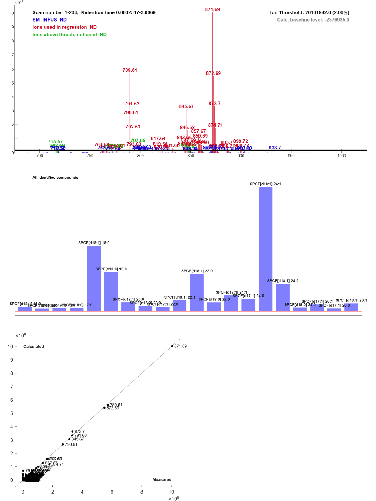
You can now press the
[LSSR Win]button in the main window. The resolved solution should look approximately like in Figure 2.4.
The sphingomyelins have masses from approximately 700 to 900 AMU. In this region there are a few minor ions marked red. There are ions that are above the threshold, but that is not accounted for by the library. Their presence indicates that the sample is not pure sphingomyelin, or thst the sphingomyelin contains other sphingoid bases or fatty acids than those in the default lists.
By right-clicking on the bars or the labels in the bar plot you get information about each compound and you can search Lipid Maps or other bases to verify that these are common sphingomyelins, or get alternative identifications, by right-click in the information field.
The predicted versus measured plot shows that most masses are close to the 1:1-line, which indicates good accuracy. But there are a few ions that have a zero measured value and a calculated value above zero. The largest of these are 791.62. If you right-click on the label in the plot you will be told that this ion appears in SPCF[d18:1] 18:0.
Close the LSSR window by pressing the
[Close]button.
2.5. Using the library as a filter.
Once a library that fits the data is generated you can also use the library as a filter when the data are imported.
Open the window for reading chromatographic data by pressing
[Import Chrom]and selectmzXMLas the file type. Select\Tutorial-2andSM_INFUSagain, as explained in 2.1Set
Resolutionto0.01andMass offsetto-0.001, turn the mean filter on and the max filter off, and Import the data by pressing[Load Sel.].Select
Avg Spectras view to display the loaded spectrum.Select thereafter
Library filterin the right table and press[Recalc Sel.]. This will filter away ions that are not in the library and the result is a spectrum of the sphingomyelins.Press
[Accept]to go back to the main window and press the[LSSR Win]button again.
This should give similar results as the previous solution, but with a cleaner spectrum.
Tutorial 3. The Lipid Gerator
The purpose of this tutorial is to give an overview of the lipid generator.
3.1. Basics
The lipid generator generates lipid compounds by combining lists of common lipid classes, common fatty acids, and common sphingoid bases. However, there are lipid compounds that are not covered, either because the entire lipid class is not implemented or because they require fatty acids or sphingoid bases that are not in the default lists.
Because the lipid generator creates every combination of the active classes and compounds it will also generate compounds that does not occur naturally. Which compounds that are generated can to a large extent be controlled by setting weights for the different compounds or by activating or deactivating fatty acids or sphingoid bases for each lipid class.
The molecular formula for the compounds in the lists are given in the fully hydrolyzed form, and the lipid compounds are built by condensation reactions, i.e. for each linkage formed, the molecular formulas of the fragments are added and a water molecule is subtracted. The exception is when ether and vinylether bonds are formed, where O2 and H2O2 are subtracted, respectively.
3.2. Codes
Glycerolipids have the following convention for naming: The letter G denotes that the molecule contains a glycerol, P denotes that it contains a phosphate group. The letters C, E, I and S denote choline, ethanolamine, inositol, and serine, respectively. A number following any of the letters denotes the total number of the group if it is more than one. Numbers in brackets denote how many fatty acids that are found in the molecule. If the number in brackets is followed by o or p it denotes that one of the fatty acids is bound by an ether or vinylether bond, respectively. The bracket is thereafter followed by a specification of the fatty acids, either as total number of carbons and total number of double bonds, denoted by t, or specified for each position, where letters a-c denotes sn-1 to sn-3 position in the glycerol, and x denotes an unknown position. Fatty acids with an additional oxygen (e.g. hydroxy or methoxy fatty acids) are denoted by +O following the number of double bonds.
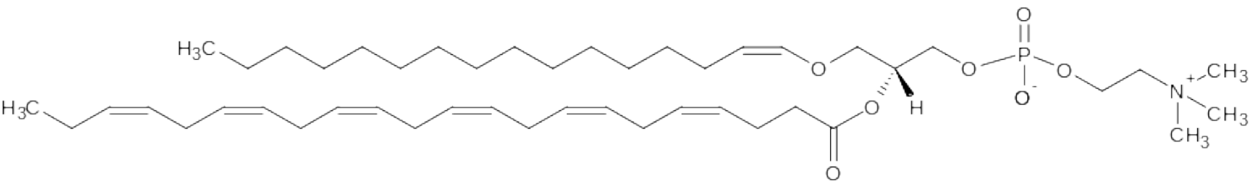
In this system the compound in Figure 3.1 can be described in several ways with different levels of detail:
GPC[2p] t32:0 – The compound has two fatty acids with a total of 32 carbons and 6 double bonds, and one of the fatty acids is bound by a vinyl ether group.
GPC[2p] x16:0 x22:6 – The two fatty acids are 16:0 and 22:6 but the positions are unknown.
GPC[2p] ap16:0 b22:6 – 16:0 is in sn-1 position and 22:6 is in sn-2 position, and 16:0 is linked by a vinylether bond.
GPC[2p] ap16:0 b22:6(4,7,10,13,16,19) – Same as above but with double bond positions specified.
Alternative 1 is applied by the lipid generator, but if more details about the structure are known, the compounds can be further specified by alternatives 2-4 within the same system.
Most sphingolipids contain a single fatty acid in addition to the sphingoid base. The naming convention for the sphingolipids is therefore the following:
The letter S denotes that the molecule contains a sphingoid base. The letters C, E, I and S have the same meaning as for the glycerolipids. G and M denotes galactose and mannose units, respectively. Since G is also used for glycerol it is important that is it specified as the first letter in the code if it refers to glycerol. To account for hydrolyzed forms that contain no fatty acid, an F is added as the last letter if a fatty acid is present (in glycerolipids this can be handled by a zero in the bracket)
The bracket in sphingolipids refers to the type of sphingoid base. The numbers in brackets are the total number of carbons and double bonds in the base, and the letter d or t preceding the number denotes two or three hydroxy groups in the base, respectively. The bracket is followed by the number of carbons and double bonds in the fatty acid.
There are some additional classes. Although platelet activation factor can be described as a phosphocholine with an ether bond (GPC[2o]) and an esterified C2 fatty acid, it is defined as a separate group named PAF. Free fatty acids are named F[1]. Cholesterol is not in the current compound list but is denoted by C[0] or as C[1] followed by the fatty acid if esterified.
The complete list of compound classes with structures and examples are given in Appendix 1 at the end of the document.
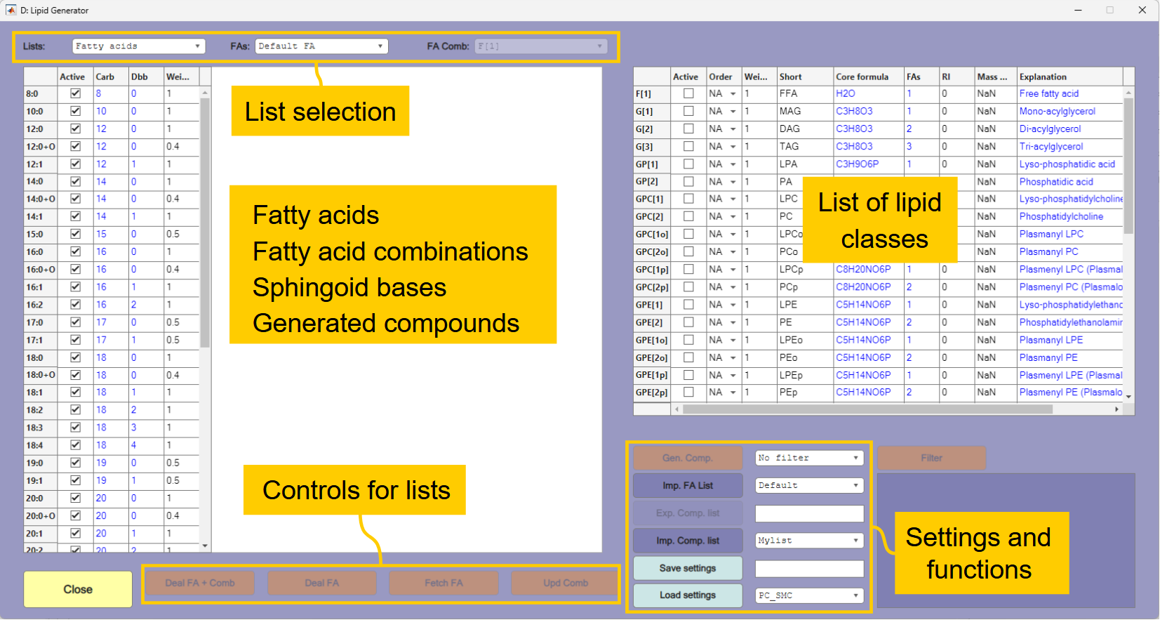
3.3. Main functions of the generator
The lipid generator window is shown in Figure 3.2. The list of lipid classes that can be generated is shown in the table to the right in the window. The table to the left shows the fatty acid list, fatty acid combinations, sphingoid bases or generated compounds. The fatty acid list is displayed when the window is opened. The list to display is selected in the list selection area. Below the list there are various controls that will change depending on the list shown.
Select
Fatty acid combinationsas the list to display and selectG[2](diacylglycerols) as the list to display. This shows total number of carbons and double bonds for possible combinations of the fatty acids in the default fatty acid list. The first entry is 16:0 because 8:0 is the shortest fatty acid in the list, and a diacylglycerol contains two fatty acids. If you selectG[3](triacylglycerols) the first entry will be 24:0 (3×8:0).If you select
Sphingoid basesthe default list of sphingoid bases will be shown, and if you selectCompoundsthe list should be empty because no compounds are generated yet.
3.4. Generation of compounds and filtering
Assume that you have been analyzing a mixture of phosphatidyl choline (CPC[2]) and phosphatidyl ethanolamine (GPE[2]) and would like to generate a library for these compounds.
Set
CPC[2]andGPE[2]asactivein the list to the right. Selection of classes can be done by clicking in theactivefield in the list, but if many classes are selected it is more convenient to right-click in the table and selectingList viewand then select the classes by the[Ctrl]key and the left mouse button. The same applies to selection in other lists.When the right classes are selected, press the
[Gen Comp.]button that will generate 316 compounds of each class and display the compound list. The list is sorted according to the molecular mass and you can see that there are isomeric compounds in the list because a PE molecule has the same molecular formula as a PC with three less fatty acid carbons. The first of these pairs appears at 565.73 amu (GPC[2] t20:0 and GPE[2] t23:0).
You can also see that the molecules have different weights. The weights are inherited from the weight given to the fatty acids in the fatty acid list. All fatty acids with an odd number of carbons have a weight of 0.5 and all fatty acids with an additional oxygen have a weight of 0.4. Other fatty acids have a weight of 1. The molecule GPE[2] t23:0 must contain one odd-numbered fatty acid and one even numbered fatty acid and therefore got the weight 1×0.5=0.5. The compound GPE[2] t24:0+O2 at 611.75 amu has a weight of 0.16 because it contains two oxygenated fatty acids (0.4×0.4). Compounds with an additional fatty acid oxygen and odd number of fatty acid carbons have weights of 0.2 (0.4×0.5). If you scroll down the list to 1000.57 you will see that GPE[2] t54:0 has a weight of 0.25. Even though this compound has an even number of fatty acid carbons, the only combination of the fatty acids in the list that can explain 54:0 is two 27:0 fatty acids.
Some methods for identification will require a compound list with unique molecular formulas. The generated lists can therefore be filtered. Select
Weightsnext to the[Filter]button and press the button. This will remove the isomers with the lowest weights. The compounds that were removed will be listed as isomers to the right in the compound list. Note that the majority of the compounds that were removed contain odd-numbered or oxygenated fatty acids that are rare in Nature compared to normal fatty acids with even number of carbons. These are therefore considered less likely to appear in a sample.
The weights in the fatty acid list can be edited by the user. The weights can also be edited in the list of fatty acid combinations. This may for instance be necessary to do if you apply internal standards with odd-numbered fatty acids, to ensure that the standard is not deleted. The list of isomers may tell you about possible interferents with the standard. To ensure that a certain compound is always preferred you can set the weight higher than 1.
In the list of lipid classes there is a field called
Orderthat can be edited by the user. If two isomeric compounds have the same weight the one that was generated first (lowest order) will be kept by the filter. There is also an option to filter only by the order.You can also set weights of compound classes. Assume that you would like to give preference to PC over PE. This can be done by downweighting PE. Set the
weightof PE to 0.3 in the lipid class list, press[Clear list]under the compound table and set the filter option back toNo filter. Press[Gen. Comp.]again. You will now see that PE compounds have a maximum weight of 0.3. GPE[2] t20:0+O has a weight of 0.12 (0.3×0.4×1) that is inherited from the PE class and the two fatty acids. If you filter by the weights again you should see that the compounds that are removed all belong to the PE class.
If you want further information about possible isomers you can search for isomers of the compound selected in the compound list in LipidMaps, EMBL or ChemSpider by using the popup-menu below the list.
3.5. Editing lists for each class
Assume that you have analyzed phosphatidyl cholines and know that you have some plasmalogens with ether or vinyl-ether bound fatty acids. You may also know that usually you will only find 14:0, 16:0, 18:1 and 20:4 fatty acids in plasmalogens in the sample type you are working with. In this case it does not make sense to create all possible plasmalogens from the default fatty acid list. You can solve this in the following way:
Close the lipid generator window and open it again to reset all settings.
Select the fatty acid list for the GPC[2o] class (phosphocholine with one ether linked fatty acid). Right-click and select
List view. Select14:0, hold down the[Ctrl]key and select16:0,18:1and20:4. Select theGPC[2p](phosphocholine with one vinylether linked fatty acid) and repeat the process for this class. Select the default fatty acid list again and thereafter the two class specific lists to verify that the selections are correct. SelectGPC[2],GPC[2o]andGPC[2p]in the lipid class list and press the[Gen. Comp.]button. This should generate approximately 300 ordinary PC compounds from the default fatty acid list and 10 compounds in each of the two other classes from the specific lists.
You can also select the compounds at the fatty acid combinations level. Select
FA combinationsin the list selector and display the list for theGPC[2p]class. Deselect one of the entries, select the compounds list and press[Clear list]. Generate the compounds again and verify that there are now only nine compounds generated for the GPC[2p] class and that the number of compounds for the two other classes are the same.
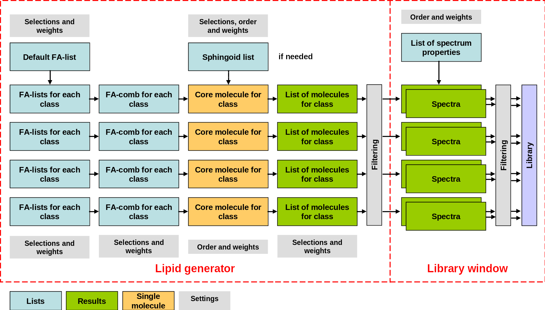
The hierarchy of the different lists and functions is illustrated in Figure 3.3. Fatty acid lists for the specific classes are generated from the default fatty acid list, the fatty acid combinations (1 to 4 fatty acids) are thereafter generated from the fatty acid lists. The fatty acids are combined with the core molecule, and a sphingoid base the case of sphingolipids. The generated lists of molecules can be filtered (optionally) and thereafter saved to be used in the library function. Because there is a separate filtering step in the library function, unique spectra can also be generated from unfiltered compound lists.
The fatty acid lists for each class is generated from active compounds in the default fatty acid list the first time the list for a class is displayed or used to generate lipids. The same applies for the combination lists. So if lipid classes are generated one by one, any edits to the default list will affect which compounds that are generated for each class. The controls for the different lists are described below:
If the default fatty acid list is shown:
[Deal FA]will update all the class specific fatty acid lists according to the selections and weights of the default list.[Deal FA + Comb.]will update all the class specific lists according to the selections and weights of the default list and update the combination lists.
If a specific fatty acid list is shown:
[Fetch FA]will update the displayed fatty acid list according to the current default list.[Upd Comb]will update the combinations list according to the displayed fatty acid list.
If a fatty acid combinations list is shown:
[Calc from FA]will update the combinations list according to the current fatty acid list for the class.
If the compound list is shown:
[Del Sel.]deletes the selected compound.[Clear list]deletes all compounds.Popup menus to search for a the selected molecular formula or for sorting the list are also displayed.
3.6. User defined fatty acid lists
The default list of fatty acids may not be suitable for all sample types. User defined lists of fatty acids can be created and are stored in the libraries folder as semicolon delimited csv files with the file names falist_......csv. The number of carbons and double bonds must be specified. Optionally you can also specify additional oxygens, the weight, and whether the fatty acid is set as active or not by true / false or 1 / 0. If nothing is specified the default settings are no additional oxygens, weight 1, and active. An example of a fatty acid list opened in a text editor is shown below.
xxxxxxxxxxCarb; Dbb; Add O; Weight; Active6;0;0;1;true8;0;0;1;true10;0;0;1;false12;0;0;1;true12;1;0;1;false14;0;0;1;true...
Assume you are analyzing triacylglycerols in vegetable oil. The G[3] class will generate more than 1000 compounds when used with the default fatty acid list. Many of these will not be naturally present in vegetable oil and can lead to incorrect identifications and poor quantification.
You can select the list
Vegoilnext to the[Imp. FA list]and press the button. This list will only generate 263 compounds that is more likely to be found in vegetable oils.If you have already generated the compounds with the default fatty acid list it is important that you clear the list of compounds and press
[Deal FA + Comb]after the fatty acid list is imported before you generate a new list of compounds. This will update the data lists for the classes. Alternatively you can close and open the window again to clear old data.
3.7. Saving and loading settings and compound lists
The generated compounds can be saved in two formats. Both these formats can be read by the library function.
You can save the list and all settings by selecting a file name next to the [Save Settings] button. This will save all lists with selections and weights at the time you press [Save Settings]. It is a good option if you have created a compound list based on other than the default settings and want to save all your modifications.
The other option is to save the data as a compound list in csv format that can be edited. These are saved in the libraries folder as cmplist_... .csv. An example of a compound list is shown below:
xxxxxxxxxxCode;Formula;ShortName;Class;Weight;RI;MassoffsetG[3] t18:0;C21H38O6;TAG 18:0;G[3];1;18;NaNG[3] t20:0;C23H42O6;TAG 20:0;G[3];0.5;20;NaN...
Code, formula, short name, class and weight must be specified. Other fields are optional. A user defined list does not have to follow conventions for names and classes used by the lipid generator. Note that atoms in the molecular formula should be given in the order H, D (deuterium) ,C, Cl, N, Na, O, P and S. Other atoms are currently not handled.
You can mix user created lists and lists generated by the lipid generator. Close the lipid generator and open it again to reset all settings. Select the list
Mylistnext to the[Imp. Comp. List]button and press the button. This will import an experimental compound list with 96 PC and PE compounds. If you filter it you will see that two of the molecular formulas have isomers. Since all weights in this case are one, the compound that was specified first in the imported list is preferred, and the other compound is listed as an isomer.Select the default fatty acid list and deactivate all fatty acids with an additional oxygen (these are not present in the imported list) and thereafter press
[Deal FA + Comb.].Select the classes
GPC[2]andGPE[2]in the lipid class list. Ensure that filter is set toNo filterand press[Gen. Comp.]. This will add approximately 560 new compounds to the list. Set the filter toOrderand press the[Filter]button.
This will give you a filtered list consisting of both imported and generated compounds. If the imported compounds are covered by the generated compounds the name will be from the imported list and the generated compounds are shown as isomers. If an imported compound has no isomers it means that it is not covered by the generated compounds (such as PC28:6 at 665.85 amu). If the fatty acid composition of your sample is known you can use this procedure to create a fatty acid list and verify the experimental identifications. A compound that cannot be explained by the fatty acid composition of the sample is not correctly identified.
3.8. Sphingoid bases
Because sphingolipids can vary in number of carbons and double bonds both in the fatty acid and in the sphingoid base, activating the full list of sphingoid bases will create a lot of isomers. The common sphingomyelin SPCF[d18:1] 16:0 (C39H79N2O6P at 703.04 amu) can for instance have the following isomers: SPCF[d17:1] 17:0, SPCF[d18:0] 16:1, SPCF[d17:0] 17:1, SPCF[d20:0] 14:1, SPCF[d20:1] 14:0, SPCF[d14:1] 20:0 and SPCF[d16:1] 18:0. To reduce the number of isomers, only the following sphingoid bases are set as active by default:
d18:1 (Sphingosine)
d18:0 (Sphinganine)
t18:1 (Dehydrophytosphingosine)
d17:1 (C17 Sphingosine)
d17:1 is set with a weight of 0.85, which is higher than the default weight of fatty acids with odd number of carbon atoms (0.5). This means for instance that SPCF[d17:1] 16:0 is preferred over SPCF[d18:1] 15:0. For reasonable identifications based on the molecular mass alone it is therefore important to consider whether one can expect that odd-numbered sphingoid bases are more likely than odd-numbered fatty acids, and adjust the weights if necessary.
d18:1 (Sphingosine) and d18:0 (Sphinganine) are the most common sphingoid bases, and it can be a good approach to test an unknown sample first with only these two activated to check if they adequately explains the data.
Tutorial 4. The profile analyzer
The puropose of this tutorial is to give an introduction to the Profile Analyzer that will be applied also in Tutorials 5 and 6.
4.1. Initialization
Start Chrombox D
Press
[Import Spec]Set
Masshunter XMLas file typeSelect
\Tutorial 4and read the fileLR_Prof_PC_Brain.xmlby pressing[Load Sel.].
This is a low resolution profile spectrum of porcine brain phosphatidyl choline.
Press the
[Analyze Prof.]button at the bottom of the Import Spectra window. This will take you to the Profile Analyzer
The Profile Analyzer resolves the spectrum into individual peaks and is used for the following purposes:
Centroiding of profile spectra
Quantification of profile spectra
To find models that describe shapes and positions of each peak in a profile spectrum
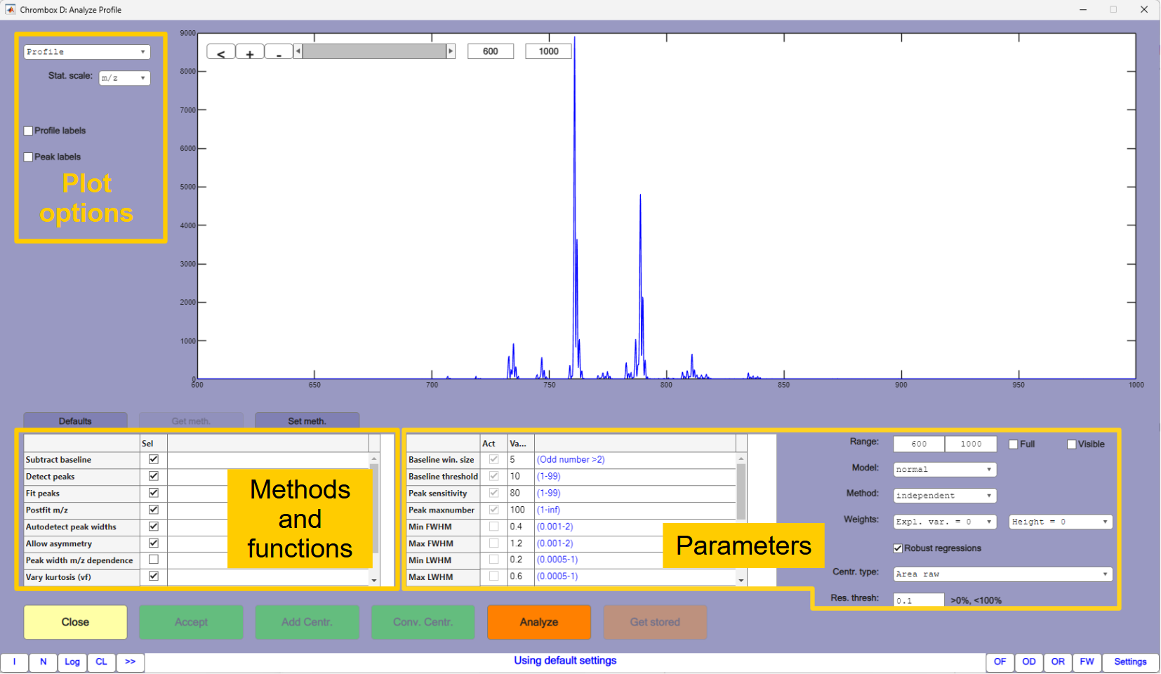
This tutorial will give an introduction to the Profile Analyzer, and you will use it to create a centroided spectrum that can later be resolved by LSSR. The Profile Analyzer window is shown in Figure 4.1.
4.2. Description of functions
At the bottom left there is a table of check boxes that controls which methods and functions to apply to the spectrum, and the associated parameters for the different functions are given in the field to the right. A summary of the functions are given below:
Subtract baselineestimates the spectrum baseline and subtracts it. The baseline is found by comparing a smoothed spectrum with the raw spectrum and the parameterBaseline win. sizesets the size of the smoothing window in data points. A value of 5 should be appropriate in most cases, but it can be beneficial to increase it if there are many data points per peak. If the value is too high compared to the number of data points per peak it may detect baseline points at peak maxima, where the peaks have slope near zero. Such points will usually be filtered, but the detection algorithm may fail if there are many such points.Baseline thresholddecides how the baseline is estimated from the data points assumed to be at baseline. A lower value will elevate the baseline. The baseline points are shown as small black dots in the spectrum, and the estimated baseline is shown as a black line. The best way to find the parameters to use is by visual inspection of these.Detect peaksdecides if the analyzer should also perform peak detection. There are two parameters that affects the detection,Peak sensitivityandPeak maxnumber. A higher value for the sensitivity may detect more peaks, until the maximum number set byPeak maxnumberis reached. Detected peaks are shown by green markers. Clicking on these will display the m/z value and the height.Fit peaksdecides how the peak models should be estimated. This is done by iterative algorithms, and which algorithm to use is determined by theMethodparameter, which can be set toindependent,regression,alternating globalorglobal.When
Methodis set toindependent, each peak will have its own peak model. This will usually give the best fit to the raw spectrum, and should be used for instance for centroiding or direct quantification based on the peak models. Because peaks may be overlapping, which cause interference, the peak fitting is run several times, using the estimates from the previous round as new start estimates.regressionalso applies individual peak fitting and use the same algorithm asindependent, but after the models have been calculated in each round they are updated with a common model for all peaks that is calculated by regression on the individual peak descriptors.globalandalternating globaltry to describe all peaks with a single model. This will usually give a poorer fit to the raw data thanindependentbut it may be a better choice if a general model for the peak shapes in the spectrum is more important than the quantitative accuracy.Another important parameter is the
Modelthat can benormal(Gaussian peaks),cauchy(Lorenzian peaks) orvoigt, which is a mixture of Lorenzian and Gaussian models. Theare are also combination models likecauchy/normalwhere different models are used to describe the left and right side of the peak (left specified first).
Postfit m/zdoes a separate optimization of the peak position after the models for peak shapes have been found. Thus, it provides better accuracy for mass determination.Autodetect peak widthswill apply initial peak widths from the peak detection algorithm. These estimates may be poor if there are few data points per peak. If the option is unchecked, the algorithms will test peak widths within the range specified by min/maxFWHM,LWHM, andRWHM, which means that there parameters should be set properly.Allow asymmetryallows the peak models to be asymmetric. Unchecking the option will speed up the algorithms, but it will usually give poorer fit to the raw data. If checked, allowed peak width range is specified by max/minLWHMandRWHM(left and right width at half maximum in mass units). If unchecked, allowed peak width range is specified bymax/min FWHM(full width at half maximum).Vary kurtosis (vf)allows peaks to have kurtosis in the case of Gaussian profiles, and it allows the degree og "Cauchyness" to vary in the case of a Voigt model. It has no effect on Cauchy models. The parameters min/max kurtosis (vf) sets the limits for the models. In the case of Voigt models, a vf of 0.5 implies a pure Gaussian model, and a vf of 1.5 implies a pure Cauchy model.Peak width m/z dependenceandKurtosis m/z dependenceallows the global peak models to be dependent on mass. If unchecked the models will be the (robust) mean of each individual peak, if checked, the peak widths and kurtosis/vf can be linearly increasing or decreasing with mass. These parameters have no effect on the individual peak profiles fitted byindependent, but it will affect the global model calculated from the individual peaks.Resolve shoulderssplits peaks detected with shoulders if this gives a significant reduction of the residuals.The other parameters are the following:
Max iterationscontrols the maximum number of iterations in iterative procedures. Decreasing the value may give faster optimization, but on the cost of accuracy.Stop criterionis a general setting for how similar results must be before the iterative methods will be stopped. Increasing the value may give faster optimization, but on the cost of accuracy.Roundsare the maximum number of rounds applied in the independent and regression procedures. Note that the maximum number of iterations in these procedures is theMax iterationsparameter divided byRounds. So settingRoundstoo high may have a negative impact on accuracy.Shoulder sens. is the sensitivity for the shoulder detection function. Higher values increase the sensitivity (more peaks may be regarded as having shoulders).Weights can used to increase the importance of peak height and the explained variance in the regression models. A weight of 0 means that all peaks have equal influence.
4.3. Using the functions
This section will teach you how to work with different functions and plot options.
In the table to the left you should deselect all functions and thereafter press the
[Analyze]button to remove all data about the spectrum.Thereafter check
Subtract baselineand press[Analyze]again. You will now have an estimate for the baseline. If you selectspectrum datain the plot options you will see the equation describing the baseline.Go back to the
Profileplot, check theDetect peaksoption and press[Analyze]. The green dots mark where the peaks were detected. You can increase number of peaks by increasingpeak sensitivityfor instance to 85. If you choose the plot optionPeak datayou will get the data for each peak, with preliminary estimates of mass, width and height.Go back to the
Profileplot, check theFit peaksoption and press[Analyze]. The green profile is the sum of the peak models, the red curve is the residuals (baseline adjusted raw data minus sum of peak models). As you can see there is a significant residual under the largest peaks, which means some degree of mismatch between the raw data and the models.Improve the models by selecting
postfit m/z,Autodetect peak widths,Allow asymmetryandVary kurtosis (vf)and thereafter pressing[Analyze]. The residuals should now be much smaller. If you choose the plot optionPeak statisticsyou will see that there is a general difference between LWHM and FWHM, which means that the peaks are asymmetric. There is nothing in the plots that indicate that peak widths or kurtosis depend on mass, so the parametersPeak width m/z dependenceandKurtosis m/z dependenceshould remain unchecked. If you choose the plot optionPeak datayou will now see more detailed (and accurate) data for each peak. There are several estimates for areas and height. See section 4.5 for a further explanation of these. The spectrum data gives you the estimates for the global peak model described by LWHM, RWHM and kurtosis.You can play around with the different parameters and functions before proceeding to the next section.
4.4. Generating a centroided spectrum and resolving it by LSSR
The standard LSSR algoritm works only on centroided and binned data. In this section you will use the Profile analyzer to generate a centroided spectrum to be resolved by LSSR.
Start by setting all parameters to the default values by pressing
[Defaults]above the methods and functions table. Thereafter set thepeak sensitivityto 85 and press[Analyze].By choosing the
Centroidedplot option you will see the centroided mass spectrum. Press the[Conv. Centr.]button to convert the profile spectrum to the centroided spectrum. This will take you back to the "Import spectra" window, and a centroided spectrum is displayed on top of the profile.In the Import spectra window, check
Labelsnext toFinaland you will see that the masses have decimals. These have to be converted to integers before you continue with LSSR.Select
Bin centroidedin the dropdown menu to the left of the plot. and press[Recalc. Sel.].Verify that masses have integer values and press
[Accept].
The library you are going to use in LSSR is already made, but if you want to create it yourself the parameters are: GPC[2], GPC[2p] and SPCF lipid classes with the respective weights 1, 0.5 and 0.75, [+H]+ spectra, resolution 1 and mass offset 0.2.
Click the
[LSSR Win]button, and in the LSSR window you click the[Library]button.Next to the
[Load Libr.]button you selectTutorial-4-5and press the button followed by[Accept].Thereafter you press
[Calculate]and refine the results by pressing[Select]and[Recalc (sel)]. Verify that the two major compounds are GPC[2] t34:1 (16:0+18:1 PC) and GPC[2] t36:1 (18:0+18:1 PC).
4.5. Further description of the functions in the Analyze profile window
Baseline estimation
The procedure for finding baseline points is based on correlation between a profile estimated by quadratic functions and the raw data within a window around each m/z value in the profile spectrum. If the point is at baseline, there will be poor correlation because the data contain only noise. The parameter Baseline win size sets the window size around each point. Baseline threshold sets the sensitivity of the method. If the value is set to 10, the points with the 10% lowest correlations will be selected as initial baseline points. An iterative procedure is thereafter applied to remove points with large positive residuals (over 3 standard deviations) when a straight line is fitted through the baseline points. Finally, the baseline equation is calculated by regression on the intensities and m/z values of the remaining baseline points.
The parameters that affects the baseline are:
Baseline estimation (on/off).
Baseline win size
Baseline threshold
Peak detection
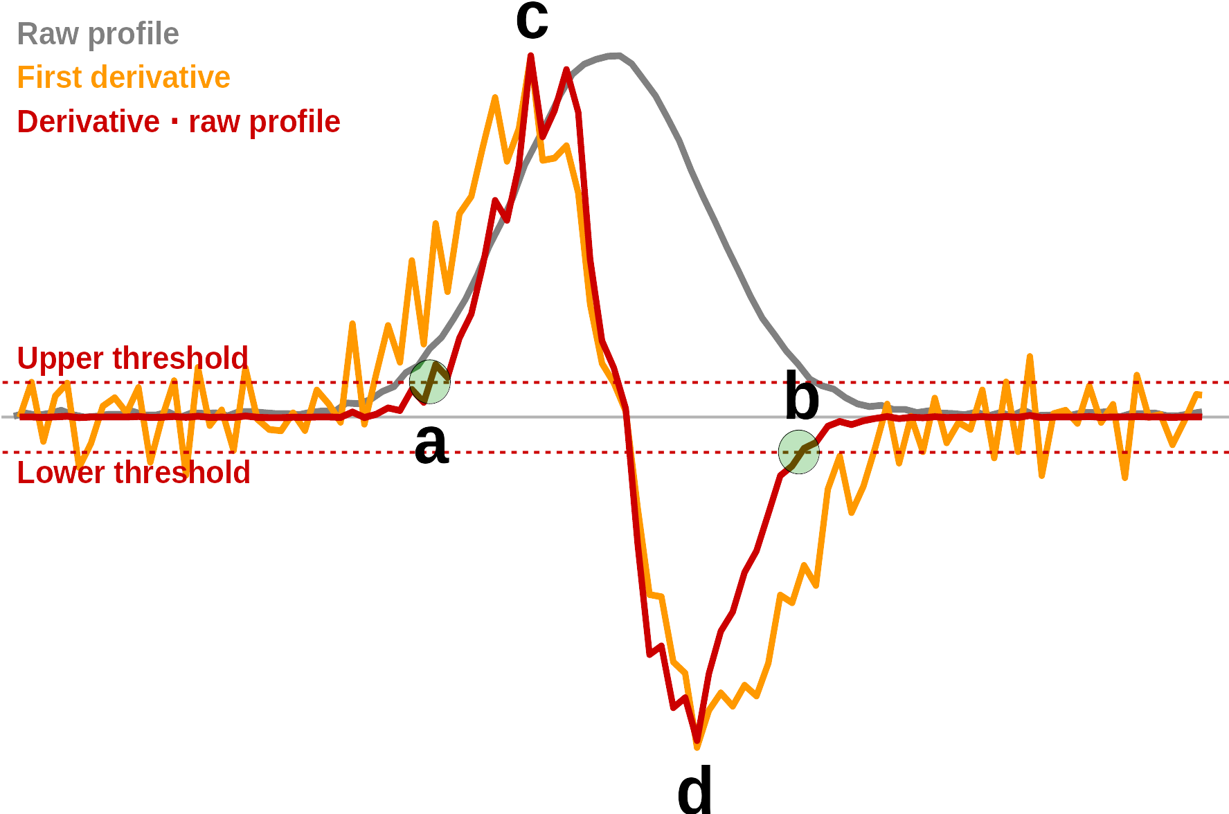
Figure 4.2 shows a normally distributed peak with some noise, the profile of its first derivative, and the profile of the first derivative multiplied with the original profile (all three profiles are normalized to same max). Peak detection is based on the derivative multiplied with the raw profile. This is less affected by noise outside peak regions than the derivative alone.
Peak starts (point a in Figure 4.2) are detected where this profile exceeds a the upper threshold, and peak ends (point b in Figure 4.2) are detected where the profile exceeds the lower threshold. After the initial peak detection there are filters for peak starts with no matching ends and ends with no matching starts. In addition the results are filtered for deviating peak widths.
Peak maxima are determined by fitting a cubic polynomial between points c and d (max/min) in the profile and solving for intensity equal to zero. The final peak widths (LWHH, RWHH) are thereafter determined on the original profile.
The parameters that affects peak detection are:
Detect peaks(on/off). If this is not selected, it is only baseline subtraction that will be performed.Peak sensitivity. This is used to set the upper/lower threshold. The upper threshold value is based on the median of of positive values in the derivative multiplied with the raw profile. This number is thereafter multiplied with 10(5-(sensitivity/20)). Since sensitivity is subtracted in the exponent, increased sensitivity means lower threshold. The lower threshold is calculated the same way, except that it is based on he median of of negative values in the derivative multiplied with the raw profilePeak maxnumber. Filter for the maximum number of peaks to detect. Set toinfto disable this filter.
Fitting of profiles
Peak profiles will be fitted to the detected peaks if the parameter Fit peaks is selected. There are several types of peak fitting. Each peak will be modelled separately if the method independent is selected. If not, the program applies a common model for the shape and widths of the profiles. There are different types of peak models that can be applied, normal (Gaussian), cauchy (Lorentzian), voigt (Gaussian/Lorentzian), and hybrid models where there are different models for the left and right side of the peak.
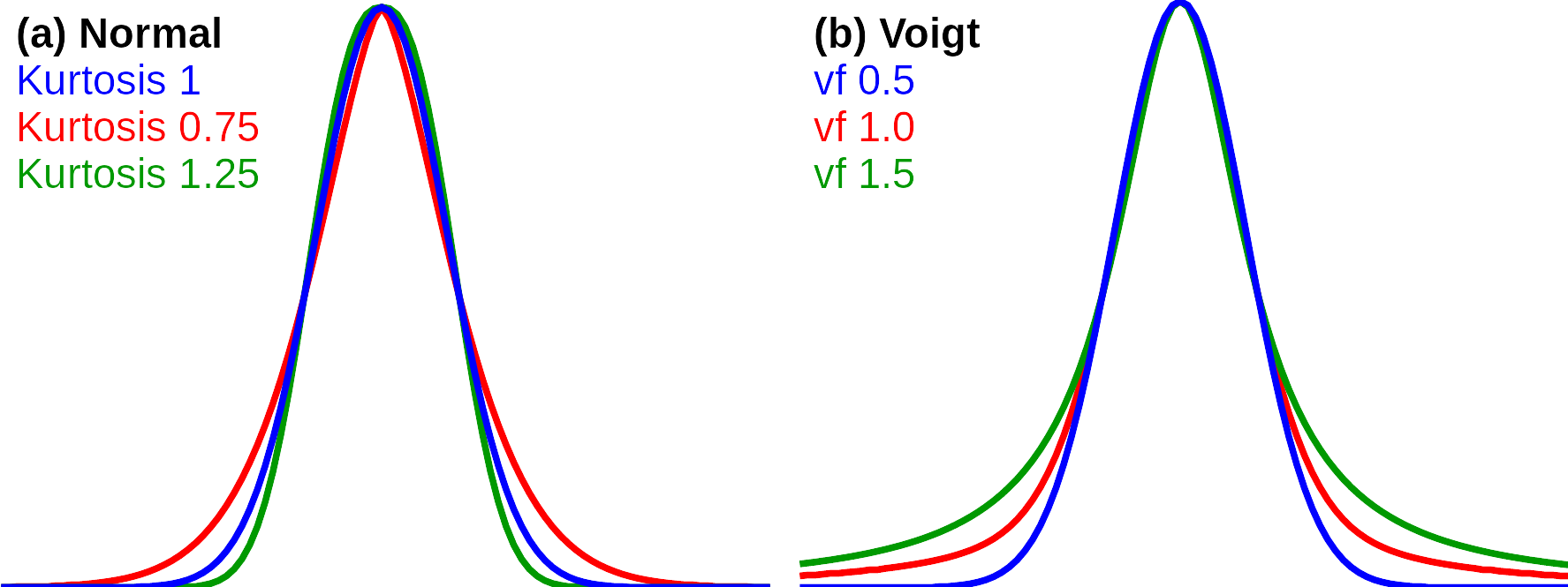
With normally distributed profiles, the program can model three parameters for each peak in addition to the position, left width at half maximum (LWHM), right width at half maximum (RWHM) and kurtosis. A kurtosis value above one means a platykurtic peak and kurtosis below one means a leptokurtic peak. With Voigt profile, the kurtosis parameter is replaced by the "voigt factor" (vf). A Voigt factor of 1.5 means that the peak is a Cauchy peak, a value of 0.5 means that the peaks is Gaussian, and values between these are mixtures of the two profile types. Normal and Voigt profiles with varying kurtosis and Voigt factors are shown in Figure 4.3. The two blue profiles are identical because both represent the normally distributed peak with no kurtosis.
The peak profiles are fitted to the raw profile by an iterative method based on the Nelder-Mead algorithm. If the option Autodetect peak widths is checked, the ranges of initial peak widths are based on the estimates from the peak detection function. Otherwise the limits for peak widths are decided by the parameters Min LWHM, Max LWHM, Min RWHM and Max RWHM if the peaks are allowed to be asymmetric (Allow asymmetry checked). The corresponding parameters for symmetric peaks are Min FWHM and Max FWHM. There are also similar settings for Kurtosis/Voigt factor.
The maximum number of iterations are set by the parameter Max iterations. There is also a stop criterion, which is a percent value (1% by default). For each iteration, the lowest residual is stored. If the development in the lowest residual for the last 100 iterations is lower than 1% of the total range of residuals, the iteration procedure is stopped.
There are four procedures for fitting the peaks. If Independent models are selected, each peak is fitted individually. The position of the peak maximum is then one of the factors that are varied in addition to the peak shape parameters. Since the fitting of a peak may be dependent on the position and shapes of overlapping neighbours it is beneficial to repeat the entire peak fitting procedure several rounds. The maximum number of rounds is decided by the Rounds parameter.
If regression or global models are selected, the optimization uses the same peak models on all peaks, but the parameters are allowed to be dependent on mass (Peak with m/z dependence and Kurtosis (vf) m/z dependence). In this case the position of one of the peaks is optimized between each iteration. The number of iterations should therefore be substantially higher than the number of peaks, so that the maximum for each peak is fitted several times.
After the iteration, the statistics for the peaks are calculated. For independent models this is done by regression on all the peaks. For global models the statistics is acquired directly from the model with the lowest residual.
Size estimates
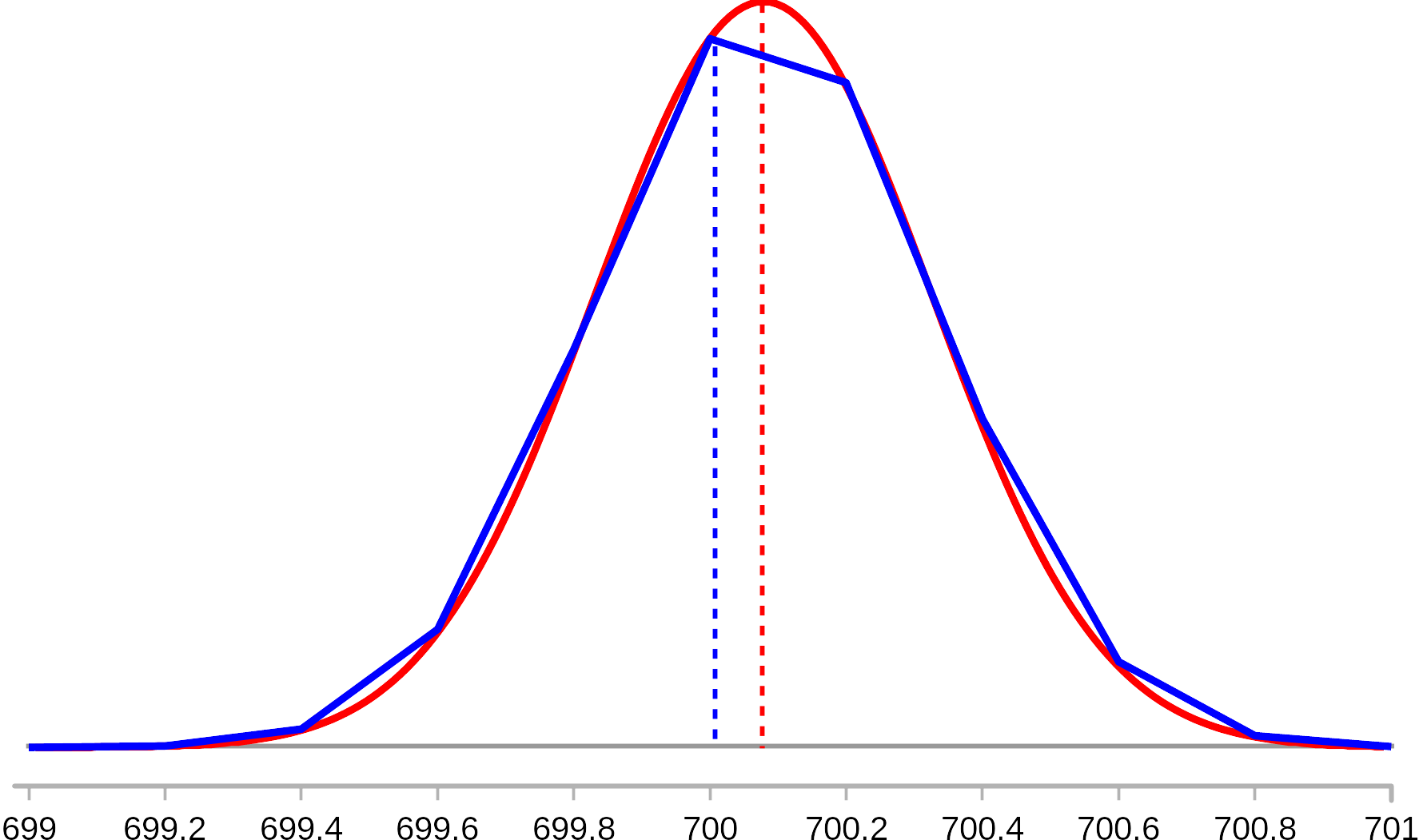
There are different ways of estimating the sizes when profiles are converted to centroids, Area raw, Area prof, Norm area raw, Norm area prof, Height raw and Height prof. The difference between the raw and prof estimates are illustrated in Figure 4.4. The figure shows an estimated peak profile (red) and this profile fitted to raw data acquired with relatively low frequency (blue). Size estimates ending with "raw" are acquired from the fit to the raw profile, and estimates ending with "prof" are estimated from the theoretical distribution. Particularly on the height estimates, there may be substantial differences between the raw and prof estimates, and the prof estimates can be assumed to be most accurate.
For estimates of areas, there are also variants starting with "Norm". This is the area multiplied with the distance between each point on the m/z scale (0.2 in figure 4.4). These areas will be independent of scan frequency.
Tutorial 5. Least squares resolution of profiles (LSSR-P)
In this tutorial you will use least squares spectral resolution (LSSR) to quantify phospholipids acquired by direct infusion mass spectrometry. The LSSR-P algorithm is an extension of LSSR for profile spectra.
5.1. Principle
LSSR was initially developed for centroided spectra, where the intensity of each peak is described by a single number. In profile spectra the peaks must be described by by vectors and the signals from the different peaks may be overlapping.
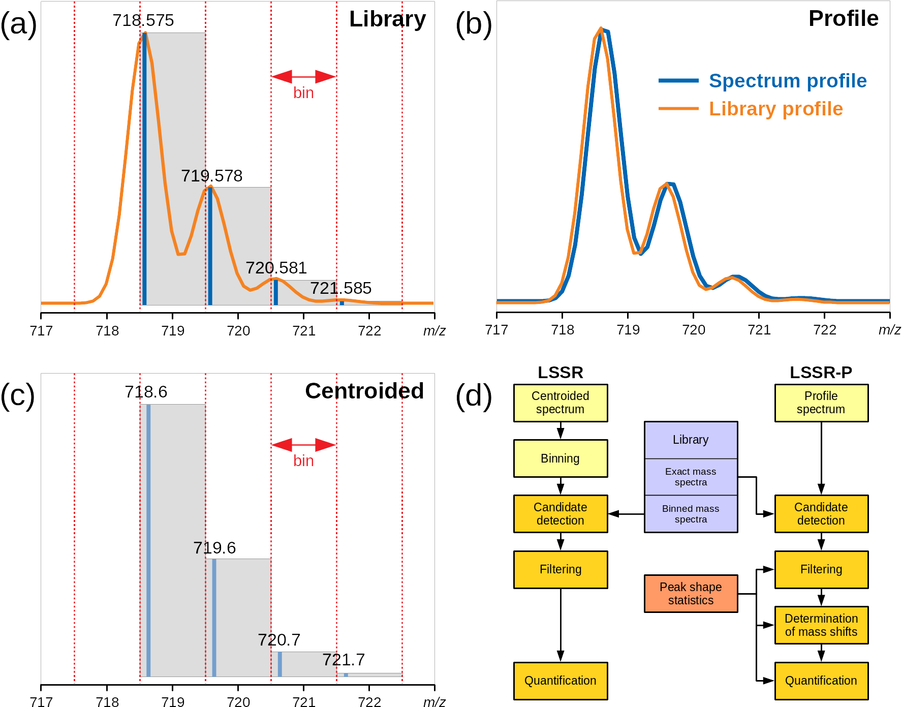
The differences between LSSR and LSSR-P are illustrated in Figure 5.1, where Figure 5.1a represents information about a single compound (PC 32:0 in this case) that is available from the library. This is the exact masses and the expected intensity of each mass.
In LSSR-P it is necessary to estimate the profiles of the library spectra and match these to the raw spectrum profile (Figure 5.1b). In LSSR for centroided spectra, the binning of both libraries and raw spectra to the same bins ensures that the mass values match, which is illustrated by the grey boxes in Figure 5.1 a and b.
To calculate the library profiles, it is necessary to know the exact masses and the expected intensity of each mass for the different compounds, which is available from the library. In addition, a model for the peak shape is needed, and this is provided by the Profile Analyzer.
The two algorithms are compared in Figure 5.1d. LSSR-P has one additional step. As illustrated in Figure 5.1b, there can be small mass shifts in the raw data compared to the exact masses provided by the library. Finding these mass shifts is handled by iterative optimization in LSSR-P, using the Nelder-Mead algorithm. The calculated shift can be equal for all compounds or they can be linearly dependent on the mass. Because LSSR-P is an iterative procedure, it is slower than LSSR. But in most cases it can be expected to be more accurate, because the centroiding and binning that is necessary for ordinary LSSR lead to loss of information.
5.2. Low resolution data
The data to be analyzed are five samples where the first four are egg PC, egg sphingomyelin (SM), bovine brain PC and bovine brain sphingomyelin, and the last sample is a mixture of the first four. The data are acquired in direct infusion mode by a low resolution triple quadrupole instrument.
The data set is stored as mz5 raw data, which must be read by the function for importing chromatograms.
Start Chrombox D and press
[Import Chrom]in the main windowEnsure that file type is set to
mz5and select\Tutorial-5. Thereafter select all 5 files and press the[Load Sel.]button. Press[Accept]when the data have been loaded.In the main window, the intensity profile of all five files are shown. Under the plot, select the
TICoption, so that only one file is shown. Ensure that this is the first file, namedLR-Prof_A_PC_Brain, which contain ordinary brain PC.To acquire the spectrum, right-click in the plot and select
Range by 20% thresh. Thereafter press[View spectrum].Right-click in the displayed spectrum and select
Analyze profile. This will take you to the Profile Analyzer.In the Profile Analyzer, press
[Analyze]without changing any parameters. SelectPeak statisticsas plot option and check that there is no pattern indicating that the residuals are mass dependent. If they show mass dependence, you should activatePeak width m/z dependenceorKurtosis (vf) m/z dependence. In this case it is not necessary. ChooseProfileas plot option again.
What is important in this case is that you get a good general estimate of the peak shapes. Whether there are some residuals on some of the peaks is less important. There is also no need to detect all peaks since you only need enough peaks to get good general models.
Since you need good general models, change
Methodtoregressionoralternating globaland thereafter press[Analyze]again. You can see the equations (baseline, LWHM, RWHM, kurtosis) for the global model by selectingSpectrum dataas plot option. Leave the Spectrum Analyzer by pressing[Accept], which will transfer the equations to the data file.
The next thing you have to do is to generate or import a library. As illustrated in Figure 5.1d, LSSR-P does not apply the binned libraries. You can therefore use the same library as in Tutorial-4, even though this is binned to unit resolution with an offset.
Press the
[Library]button in the main window. In the library window, selectTutorial-4-5next to the[Load Libr.]button and press the button. Leave the library window by pressing[Accept], which will transfer the library to the memory.Thereafter you can press the
[LSSR-P Win]button which will take you to the LSSR-P window.The only thing you have to do in the LSSR-P window is to press the
[Calc All]button, which will show you the results.
For more advanced usage you can step through the different processes illustrated in Figure 5.1 by the [Get Cand] (get candidates), [Filter Cand] (filtering), [Fit] (determination of mass shifts) and [Quantify] (quantification) buttons. In each step you can make changes in the "Candidates", "Filtered" and "Results" tables. You may for instance replace compounds in the filtered table with compounds with similar mass to see if it reduces the residuals.
Repeat the procedure with the four other samples. In the Profile Analyzer there is usually is no need to check more than one sample in the same sequence for mass dependent models, so you can directly calculate the models.
The results plots for the different samples should look approximately as in Figure 5.2. Verify that the two samples of ordinary PC contain basically PC, and that the two samples of SM contain basically SM (marked SMCi or SPCF). In the mixture (Figure 5.2e) you should find all the major compounds.
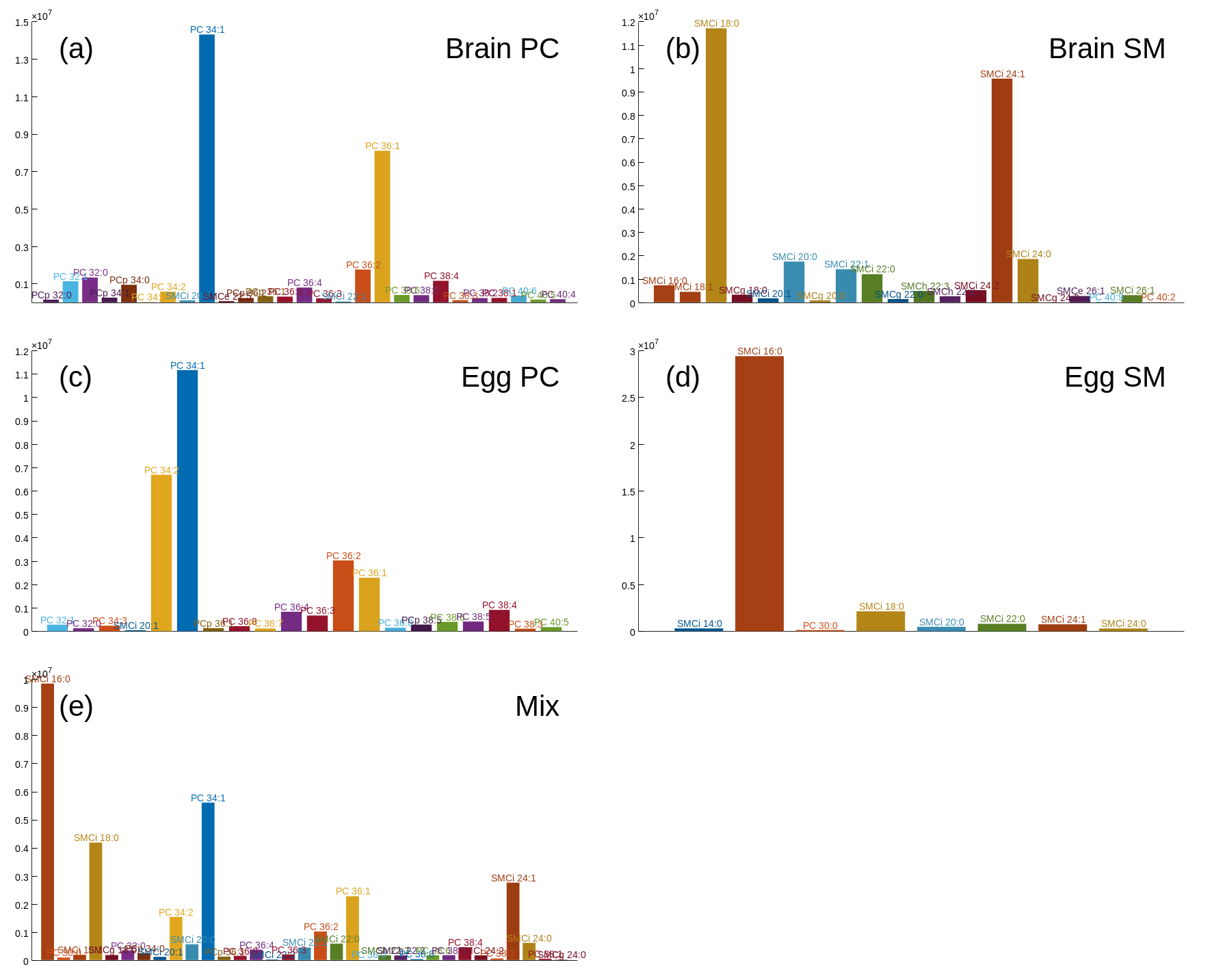
5.3. High resolution data
The same samples have also been analysed by direct infusion of a time-of-flight (TOF) instrument. In this case you read the spectra by the [Import Spec] function.
In the Import Spectra window, select
JEOL jpfas the file type, thereafter select\Tutorial-5, select all 5 files in the folder and press[Load Sel.]and[Accept]when the spectra are imported.In the main window, ensure that the first file, named
HR-Prof_A_PC_Brain, is selected, right click on the spectrum and selectAnalyze profile.
In this case the profiles are not well described by variants of the normal distribution. If you zoom on the largest peaks you will see that the peaks are asymmetric and tailing. The correct peak model to use in this case is the normal/voigt, where the left side of the peak is normally distributed and the right side of the peak has a Voigt distribution.
Select the
normal/voigtas the model to use. You can run a first test withindependentas method and check if there is any mass dependence. There should be no clear mass dependence, so you can also directly selectalternating globalbefore you press[Analyze]and leave the window with[Accept].
You can use the same library as for the low resolution data. Load the library as explained in Section 5.2 if it is not already in the memory.
In the main window, go to the LSSR-P window by pressing
[LSSR-P Win].
In this case there is a quite large mass shift compared to the width of the peaks.
Zoom in on the largest peak in the spectrum at m/z 760.712. This is the base peak of PC 34:1.
Next to the
[Library]button, check theShow Libr. Bpoption to show where the base peaks of the library spectra are located. You should then get a plot similar to Figure 5.3 a.Click on the pink line next to peak at m/z 760.712. You should then get a message in the message line at the bottom of the window telling that this PC 34:1, which has an exact mass of 760.585 Da.
The difference between the exact mass and the peak maximum is therefore −0.127 (760.585 − 760.712), which is similar to FWHM (approx 0.11). The parameter m/z shift window sets a max limit for m/z shift in percent of the peak width, and the default is 50%. You can increase this value, but it is usually better to manually adjust the m/z scale by the m/z offset parameter.
Set
m/z offsetto the difference between the exact and measured mass, −0.127. This should shift the mass spectrum to fit better with the library data. It should then look approximately like in Figure 5.3 b, where the blue curve is the shifted profile and the grey curve is the original profile.You can now press the
[Calc All]button to get the results.
You can analyze the remaining samples with the same procedure. The mass offset of −0.127 can be used for all samples. The results should be similar to those shown in Figure 5.4. There are small differences between the two instruments even though there is a large degree of overlap in the low resolution spectra. However, in general the high resolution instrument detects a few more samples and it will usually be better in cases where samples are very complex.
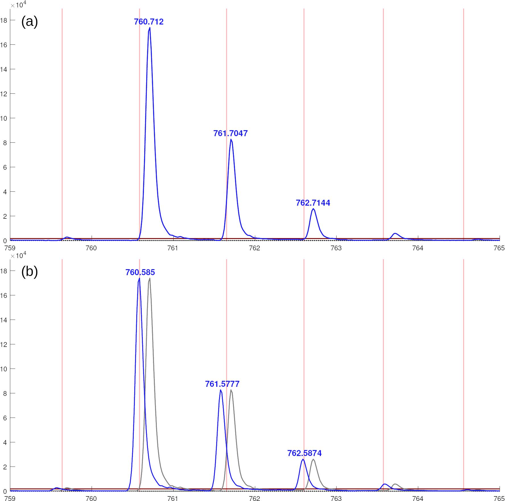
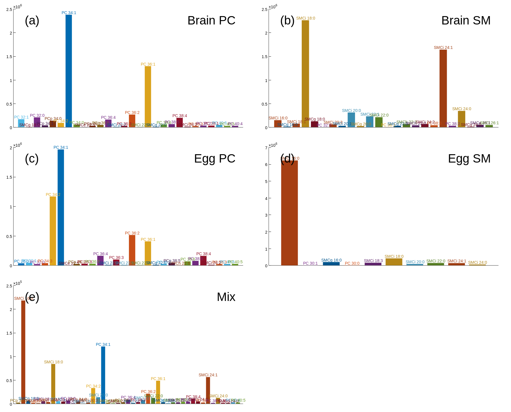
Tutorial 6. Accurate mass determination
In this tutorial you will apply the peak models from the Profile Analyzer to determine the mass of unknowns. The tutorial has two sections, one for low resolution and one for high resolution data.
6.1. Low resolution data
The data are six replicates of brain phosphocholine analysed by direct infusion on a triple quadrupole instrument. It is the same sample as applied in Tutorial 5. We therefore know that the three most abundant compounds are PC 34:1, PC 36:1 and PC 36:2. However, the sample is now spiked with the saturated PCs 24:0, 28:0, 32:0, 36:0, 40:0, 44:0, and 48:0. These will be used as reference series for the mass calibration.
Open Chrommbox D and press
Import Chrom.Ensure that
file typeismz5and select\Tutorial-6. Select all the six samples and press[Load Sel]. Return to the main window by pressing[Accept].In the main window select
TICas display option.
You will now have to apply the Profile Analyzer on all six data files in the same way as you did in Tutorial 5. The procedure for the first file is:
Right-click on the main plot and select
Range by 20% thresh.Thereafter press
[View Spectrum].Right-click in the spectrum and select
Analyze profile.
You should now be in the Profile Analyzer.
Press
[Analyze]once to ensure that you are using the right peak model. There should be almost no residuals.Thereafter change
Methodto toalternating globaland press[Analyze]again, since it is critical in this case to apply the same models on all peaks.Leave the Profile Analyzer by pressing
[Accept].
Repeat the steps above for the remaining 5 data files.
When all files have associated peak models you can press the
[Mass Calibr.]button in the main window. This will take you to the mass calibration window.Next to the [Load Libr.] button in the mass calibration window, selct Calibration and press the button. Also ensure that
Spectra: [M+H]+is selected.
You should now have a table showing the accurate masses for the library compounds, and there will be vertical grey lines in the spectrum indicating the masses of the two largest peaks from each library compound. The next step is to match these masses from the library to the peaks in the spectrum.
Press
[Match All], and all the grey lines should turn pink, indicating that they have been matched to a peak. The plot of the spectrum should look like in Figure 6.1, except for the three red arrows that indicate which peaks to work with later. You can use the[<]and[>]buttons to go through the spectra and check that all peaks are correctly matched.
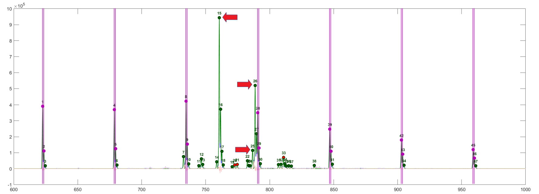
If you select
Match plotat the bottom of the table you will get a plot that explains the difference between the library masses and the matched peaks. In this case it will vary from approximately 0.16 to 0.23 mass units. Closed circles are the values for the current spectrum. Open circles are the values for the other replicates. Thi plot should look like Figure 6.2.
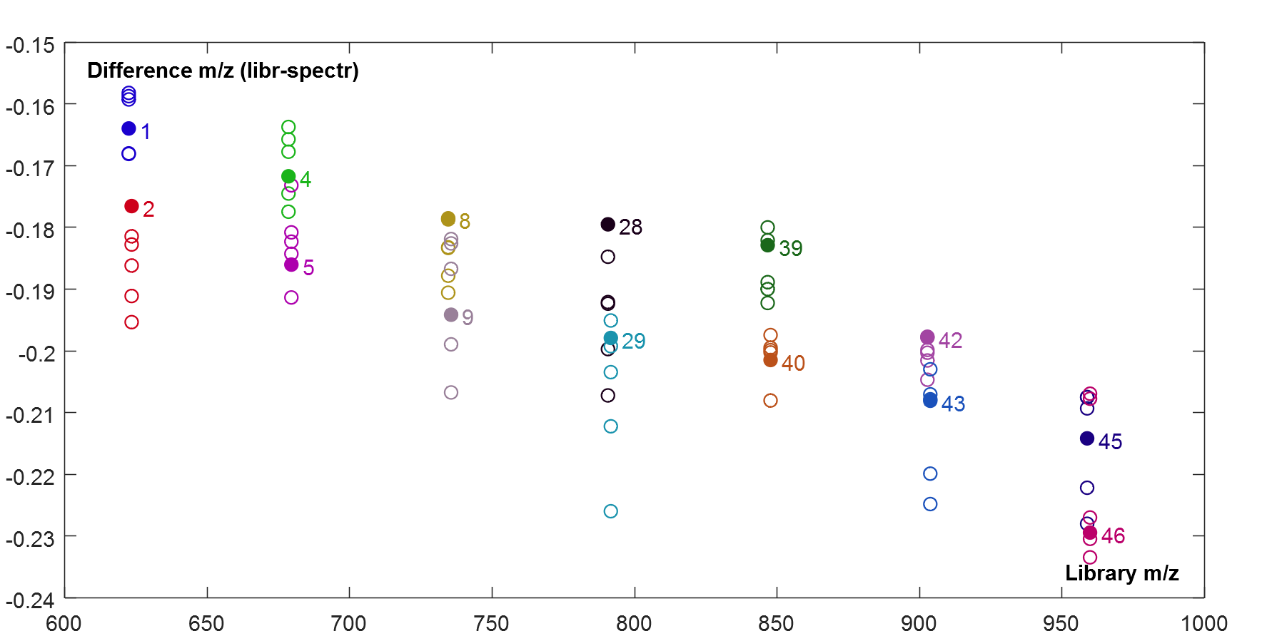
The next step is to find a regression model that explain the differences . This function will later be used to calculate the accurate masses of the other peaks in the spectrum. The plot shows that the differences are dependent on the mass and that the dependence is close to linear. We should therefore apply a linear regression model.
Ensure that the model type is set to
Polynom ord. 1in the field under the[Regression]button and also thatRobustregression is checked. Thereafter press[Regr. All].
Two regression lines will now be shown in the plot. The black is the regression model for the current spectrum. The grey is the regression line based on all the other replicates (the open circles).
You are now ready to predict the masses for the other peaks. Press
[Prediction], and a table of predicted masses will be shown.
We know from Tutorial 5 that the three most abundant compounds in the sample are PC 34:1, PC 36:1 and PC 36:2. The base peaks of these are indicated by the red arrows in Figure 6.1. We should now assume that these are unknown compounds and check the predicted masses versus the Lipid Maps database.
Click on the peak number label of largest peak in the spectrum. This should be the base peak of PC 34:1. You should now get a table similar to the one below, that contains predictions and statistics for this peak but you may have slightly different values.
| Parameter | Prediction |
|---|---|
| Raw m/z, [M+H]+ | 760.8 |
| fitted m/z, [M+H]+ | 760.7626 |
| Predicted m/z, [M+H]+ (internal calibr.) | 760.5751 |
| Predicted m/z, [M+H]+ (external calibr.) | 760.5729 |
| Predicted neutral mass (internal calibr.) | 760.5751 |
| Predicted neutral mass (external calibr.) | 759.5656 |
| Internal calibr. RMSE | 0.0095 |
| Internal calibr. median residual | 0.0066 |
| External calibr. RMSE | 0.011 |
| External calibr. median residual | 0.0075 |
| Mean neutral mass (internal calibr.) | 759.572 |
| Median neutral mass (internal calibr.) | 759.5739 |
| Number of samples, consensus estimates (internal calibr.) | 5 |
| Mean neutral mass (external calibr.) | 759.5752 |
| Median neutral mass (external calibr.) | 759.5755 |
| Number of samples, consensus estimates (external calibr.) | 6 |
There are several estimates for the mass. You can apply the Median neutral mass based on internal calibration that is shown with bold text. This is the median of all six replicates, so it is enough to acquire the statistics from a single sample. The two error estimates show how the predictions vary between the replicates. They indicate that the error may be slightly lower than 0.01 mass units.
In the following web page you can search the Lipid Maps database by mass:
https://www.lipidmaps.org/tools/ms/LMSD_search_mass_options.php
Go to the web page and paste the predicted mass (759.5739) into the field
Mass (m/z). Select all the possible lipid classes. SetIontoM(neutral)and mass tolerance to+/- 0.01and press the[submit]button on the web page. You will see that all the alternatives are variants of PC 34:1 with molecular formula C44H87NO8P. So the accuracy is good enough to identify this as PC 34:1 as long as you can assume that it is a lipid.
The accurate masses from Lipid Maps and the predictions for the three most abundant compounds are compared in Table 6.2. None of the errors were above 0.01 mass units and none of the compounds have any interference within this mass tolerance. It is worth noting that the errors are much smaller than the digital data resolution of the instrument, which is 0.1 mass units.
You can play around with the mass tolerances to see when interferents (compounds with different gross formula) appear among the alternatives.
| Accurate mass | Predicted mass | Error | |
|---|---|---|---|
| PC 34:1 | 759.5778 | 759.5739 | -0.0039 |
| PC 36:1 | 787.6091 | 787.6039 | -0.0052 |
| PC 36:2 | 785.5935 | 785.5959 | 0.0024 |
6.2 High resolution data
The high resolution data are from a time-of-flight instrument. The samples are exactly the same as used with low resolution.
To import the data, press the
[Import Spec]button, SetFile typetoJEOL jpf, select\Tutorial-6, select all six files, press[Load Sel]and exit with[Accept].Select the first data file, right-click in the spectrum and select
Analyze profile.In the Profile Analyzer, adjust the lower range to 600 since there are no peaks of interest below this mass, set
Modeltonormal/voigtand setMethodtoalternating global. This is similar settings as used in Tutorial 5.Press
[Analyze]and[Accept]to transfer the models to the data fileRepeat for all 5 remaining replicates
When all files have associated peak models you press the
[Mass Calibr.]button that opens the mass calibration window.
The procedure to analyze the high resolution data is the same as used before.
Load the library
Calibrationand press[Match All].
If you inspect the difference plot (Fig. 6.3) you will see that there is a tendency to curvature in the data, so it may be beneficial to change the model to Polynom ord. 2. If you step through the replicates using the [<] and [>] buttons you will also see that there is a tendency to drift over time.
After you have selected the regression model, press
[Regr. All]and[Prediction].
If you click on the peak numbers and compare predictions to the correct values for the same three compounds analyzed with the low resolution data you should get values similar to those in Table 6.3. The average error is approximately 1/3 of what it was with the low resolution instrument. The FWHM for the high resolution instrument was 0.10, while it was 0.65 for the low resolution instrument, which means that the peak width was more than 6 times higher for the low resolution instrument. It is therefore no direct link between resolution and the expected accuracy of the masses after calibration.
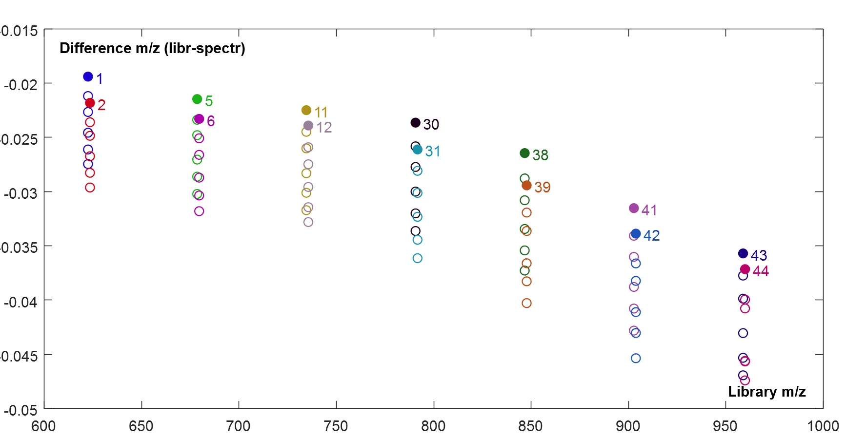
| Accurate mass | Predicted mass | Error | |
|---|---|---|---|
| PC 34:1 | 759.5778 | 759.5766 | -0.0012 |
| PC 36:1 | 787.6091 | 787.6082 | -0.0009 |
| PC 36:2 | 785.5935 | 785.5948 | 0.0013 |
Appendix 1. List of lipid classes with examples of naming
| CodeCore | Explanation / short Example |
|---|---|
| F[1] | Free fatty acid / FFA |
| H2O |  F[1] 16:0 F[1] 16:0 |
| G[1] | Mono-acylglycerol / MAG |
| C3H8O3 |  G[1] 16:0 G[1] 16:0 |
| G[2] | Di-acylglycerol / DAG |
| C3H8O3 |  G[2] t32:0 G[2] t32:0 |
| G[3] | Tri-acylglycerol / TAG |
| C3H8O3 |  G[3] t48:0 G[3] t48:0 |
| GP[1] | Lyso-phosphatidic acid / LPA |
| C3H9O6P |  GP[1] 16:0 GP[1] 16:0 |
| GP[2] | Phosphatidic acid / PA |
| C3H9O6P |  GP[2] t32:0 GP[2] t32:0 |
| GPC[1] | Lyso-phosphatidylcholine / LPC |
| C8H20NO6P |  GPC[1] 16:0 GPC[1] 16:0 |
| GPC[2] | Phosphatidylcholine / PC |
| C8H20NO6P |  GPC[2] t32:0 GPC[2] t32:0 |
| GPC[1o] | Plasmanyl-lyso-phosphatidylcholine / LPCo |
| C8H20NO6P |  GPC[1o] 16:0 GPC[1o] 16:0 |
| GPC[2o] | Plasmanyl-phosphatidylcholine / PCo |
| C8H20NO6P |  GPC[2o] t32:0 GPC[2o] t32:0 |
| GPC[1p] | Plasmenyl-lyso-phosphatidylcholine (LPC plasmalogen) / LPCp |
| C8H20NO6P |  GPC[1p] 16:0 GPC[1p] 16:0 |
| GPC[2p] | Plasmenyl-phosphatidylcholine (PC plasmalogen) / PCp |
| C8H20NO6P |  GPC[2p] t32:0 GPC[2p] t32:0 |
| GPE[1] | Lyso-phosphatidylethanolamine / LPE |
| C5H14NO6P |  GPE[1] 16:0 GPE[1] 16:0 |
| GPE[2] | Phosphatidylethanolamine / PE |
| C5H14NO6P |  GPE[2] t32:0 GPE[2] t32:0 |
| GPE[1o] | Plasmanyl-lyso-phosphatidylethanolamine / LPEo |
| C5H14NO6P |  GPE[1o] 16:0 GPE[1o] 16:0 |
| GPE[2o] | Plasmanyl-phosphatidylethanolamine / PEo |
| C5H14NO6P |  GPE[2o] t32:0 GPE[2o] t32:0 |
| GPE[1p] | Plasmenyl-lyso-phosphatidylethanolamine / LPEp |
| C5H14NO6P |  GPE[1p] 16:0 GPE[1p] 16:0 |
| GPE[2p] | Plasmenyl-phosphatidylethanolamine (PE plasmalogen) / PEp |
| C5H14NO6P |  GPE[2p] t32:0 GPE[2p] t32:0 |
| GPI[1] | Lyso-phosphatidylinositol / LPI |
| C9H19O11P |  GPI[1] 16:0 GPI[1] 16:0 |
| GPI[2] | Phosphatidylinositol / PI |
| C9H19O11P |  GPI[2] t32:0 GPI[2] t32:0 |
| GPI[1o] | Plasmanyl-lyso-phosphatidylinositol / LPIo |
| C9H19O11P |  GPI[1o] 16:0 GPI[1o] 16:0 |
| GPI[2o] | Plasmanyl-phosphatidylinositol / PIo |
| C9H19O11P |  GPI[2o] t32:0 GPI[2o] t32:0 |
| GPS[1] | Lyso-phosphatidylserine / LPS |
| C6H14NO8P |  GPS[1] 16:0 GPS[1] 16:0 |
| GPS[2] | Phosphatidylserine / PS |
| C6H14NO8P |  GPS[2] t32:0 GPS[2] t32:0 |
| GPS[1o] | Plasmanyl-lyso-phosphatidylserine / LPSo |
| C6H14NO8P |  GPS[1o] 16:0 GPS[1o] 16:0 |
| GPS[2o] | Plasmanyl-phosphatidylserine / PSo |
| C6H14NO8P |  GPS[2o] t32:0 GPS[2o] t32:0 |
| G3P2[4] | Cardiolipin / CL |
| C9H22O13P2 |  G3P2[4] t72:8 G3P2[4] t72:8 |
| SF | Ceramide / Cer (Sphingosine base) |
| H2O |  SF[d18:1] 16:0 SF[d18:1] 16:0 |
| SF | Ceramide / Cer (Phytosphingosine base) |
| H2O |  SF[t18:0] 16:0 SF[t18:0] 16:0 |
| SPCF | PC Ceramide / SMC (Sphingomyelin, sphingosine base) |
| C5H14NO4P |  SPCF[d18:1] 16:0 SPCF[d18:1] 16:0 |
| SPCF | PC Ceramide / SMC (Sphingomyelin, phytosphingosine base) |
| C5H14NO4P |  SPCF[d18:0] 16:0 SPCF[d18:0] 16:0 |
| SPEF | PE Ceramide / SME |
| C2H8NO4P |  SPEF[d16:1] 18:0 SPEF[d16:1] 18:0 |
| SPIF | PI Ceramide (IPC) / SMI (Sphinganine base) |
| C6H13O9P |  SPIF[d18:0] 16:0 SPIF[d18:0] 16:0 |
| SPIF | PI Ceramide (IPC) / SMI (Phytosphingosine base) |
| C6H13O9P |  SPIF[t18:0] 16:0 SPIF[t18:0] 16:0 |
| SMIPF | Mannosylinositol phosphoceramide / MIPC (Sphinganine base) |
| C12H23O14P |  SMIPF[d18:0] 16:0 SMIPF[d18:0] 16:0 |
| SMIPF | Mannosylinositol phosphoceramide / MIPC (N,N-dimethyl-Safingol base) |
| C12H23O14P |  SMIPF[d20:0] 16:0 SMIPF[d20:0] 16:0 |
| SMI2P2F | Inositol phosphomannosylinositol phosphoceramide / MIP2C |
| C18H34O22P2 |  SMI2P2F[d18:0] 16:0 SMI2P2F[d18:0] 16:0 |
| SGF | Galactosyl ceramide / GCer (Sphinganine base) |
| C6H12O6 |  SGF[d18:0] 16:0 SGF[d18:0] 16:0 |
| SGF | Galactosyl ceramide / GCer (Sphingosine base) |
| C6H12O6 |  SGF[d18:1] 16:0 SGF[d18:1] 16:0 |
| PAF[1o] | Platelet activation factor / PAF |
| C10H22NO7P |  PAF[1o] 16:0 PAF[1o] 16:0 |